Giovanni Bricconi

Reading the LSTM article on comparing different architectures (“LSTM a search space odissey”) I was curious to understand better theirs approach on identifying important parameters. They referenced this article:

An Efficient Approach for Assessing Hyperparameter Importance. Frank Hutter, Holger Hoos, Kevin Leyton-Brown. Proceedings of the 31 st International Conference on Machine Learning, Beijing, China, 2014. JMLR: W&CP volume 32.

The technique used is called f-ANOVA, which stands for functional analisys of variance. Before looking at I wanted to read a bit on simple ANOVA, just to understand a bit more: as the reading is about statistics, it was really scaring to me – really not my favourite subject.

Luckily the web is full of introductive pages; I read this one “A Simple Introduction to ANOVA (with applications in Excel)“. In a nutshell an anova example is:

A recent study claims that using music in a class enhances the concentration and consequently helps students absorb more information. We take three different groups of ten randomly selected students (all of the same age) from three different classrooms. Each classroom was provided with a different environment for students to study. Classroom A had constant music being played in the background, classroom B had variable music being played and classroom C was a regular class with no music playing. After one month, we conducted a test for all the three groups and collected their test scores.

See “A simple introduction to anova” to know how it can be done

Here the ANOVA test compare more than 2 categories (we have A,B and C groups) and checks if the average is the same or if there is a significative difference between the groups averages. If you have just 2 categories you can use a different test, and also the test itself just answers if the difference is significative, you need to dig more if this is true.

Trying to dig more, I have quickly found many references to complex statistic subjects, so I retained that it is mandatory to find a tool that does the analysis for you, otherwise the risk of making mistakes is too high and already interpreting the results it is not easy.

After that I have come back to the article on f-ANOVA, and luckily for me it was easier to understand that those on statistics.

The idea is more or less this one: we have one loss function that depends on many hyper-parameters, we would like to understand how much each parameter influences this loss function. In this way we spend more time on the important ones.

As in the previous post on searching good hyperparameters values, it is needed to approximate the real loss function f with another one f’ that can be quickly evaluated. As hyper-parameters can be continous (ex. drop rate), ordinal (number of layers), or discrete (training algorithm) they propose to use random forest models to build f’.

To understand quicky what a random forest tree is, you can read https://www.javatpoint.com/machine-learning-random-forest-algorithm . Many decision trees will be built, on each node there will be a test on an hyperparameter value, attached to each leaf there will be a prediction on f’ value c_i. The final predicted f’ is calculated averaging the c_i.

Usually what we do to tune a parameter is just explore the f values we can achieve keeping all the other hyper-parameters fixed: this is bad as we explore the response of f just locally to the fixed hyper-parameters. We do not know if with other fixed values it will be much different. Now that we have an estimated f’ we can do much better.

For instance we can chose one single hyper parameter i, and evaluate the variance of f’ on all the possible values of the other parameters. This is feasible as f’ can be computed quickly, and it turns out the result is linked to the size of the configuration space possible for the i values compared to the all possible parameter configurations. In the end you can decompose the variance V of f’ on the search space into the sum of contributions V_i of each parameter.

Once selected the most important parameter, you can even take 2 of them and plot in 3D how the variance changes, to understand how they are correlated.

This is way too hard to do without a tool. Next week I will look for existing tools for this and the hyper-parameter search, to understand if it is really feasible to do these analysis.

I continued reading the links on hyper-parameters optimization and I have found another interesting article:

Algorithms for Hyper-Parameter Optimization, James Bergstra, Rémi Bardene, Yoshua Bengio, Balàzs Ké́gl, https://proceedings.neurips.cc/paper/2011/file/86e8f7ab32cfd12577bc2619bc635690-Paper.pdf

As I saw with Ray, there are many algorithms that can be exploited, and I wanted to learn more. Is there a better way than just extracting parameters values and trying them to tune a model? The article begins with this phrase:

Several recent advances to the state of the art in image classification benchmarks
have come from better configurations of existing techniques rather than novel ap-
proaches to feature learning. Traditionally, hyper-parameter optimization has been
the job of humans because they can be very efficient in regimes where only a few
trials are possible. Presently, computer clusters and GPU processors make it pos-
sible to run more trials and we show that algorithmic approaches can find better
results

The authors suggests that choosing the hyper-parameters should be regarded as an outer loop in the learning process: in the outer loop you select the hyper parameters, in the inner you train the model, and you keep the model that provides the best results. Once selected the best hyper-parameter you can do a better training with more examples, and finally you have a model that can be exploited. It is therefore important to allocate enough resources and cpu time to the hyper-parameter selection, otherwise you will train a sub-optimal model.

But how can we do better than random or grid search? In my understanding grid and random search work in this way: you select some parameters, you train the model on some sample data (not all because it takes too much time), and you continue until your results (loss function value) do not improve much. Training the model is a very expensive step.

The “trick” is that, after some random/grid iteration, you could start building a model of the loss functions based on the prameters used and the results achieved (they do so after 30 random experiments). If this model is much less expensive than the training, you can then use some other algorithm to guess interesting parameter combinations to test, for instance using some gradient driven method. You choose the next candidate parameter combination in a better way than just extrancting a random combination.

Reality is more complicated than this, and an algorithm that wants to do so needs to take into account that there are relations between the parameters to explore. For instance the number or neurons in layer 2 makes sense only if you decide that your model will have 2 layers. Parameters can be continous (ex. drop rate), ordinal (number of layers), or discrete (training algorithm). The Authors say that the hyper-parameter configuration space is graph-structured.

The paper continues describing two approaches, one based on Gaussian Processes and antother on Parzen-estimators. With gaussian processes the loss function is modeled with gaussian variables; once the model is created, a new candidate point can be searched using exhaustive grid search, or some more complex algorithms, they refers to EDA and CMA-ES. With the Parzen Estimator approach, a reference y* loss function value is taken into account, this is not the best value obtained so far, but some quantiles away from that. The model created predict which parameter combinations will have a certain loss value, that is quite the reverse of the gaussian process where you predict the loss function that will have a parameter combination. From the experiments reported, the second approach is the one that gives bettere results (they experimented selecting 32 hyper-parameters).

The software they developed is called “Hyperopt”: https://github.com/jaberg/hyperopt

The hyperparameter optimization page on Wikipedia is full of interesting links. It will take me some time to explore them, as I am not satisfied of just having a basic knowledge on grid and random search.

I have followed randomly one of the links in open source softwares for hyperparameters optimization and I have reached Ray Tune. I was expecting some obscure tool but instead I have discovered a superb site full of documentation and examples.

Quoting them, Ray is defined as

Ray is a unified framework for scaling AI and Python applications. Ray consists of a core distributed runtime and a toolkit of libraries (Ray AIR) for simplifying ML compute

Today’s ML workloads are increasingly compute-intensive. As convenient as they are, single-node development environments such as your laptop cannot scale to meet these demands.

Ray is a unified way to scale Python and AI applications from a laptop to a cluster.

With Ray, you can seamlessly scale the same code from a laptop to a cluster. Ray is designed to be general-purpose, meaning that it can performantly run any kind of workload. If your application is written in Python, you can scale it with Ray, no other infrastructure required.

https://docs.ray.io/en/latest/index.html

I have just looked a bit into the Tune module:

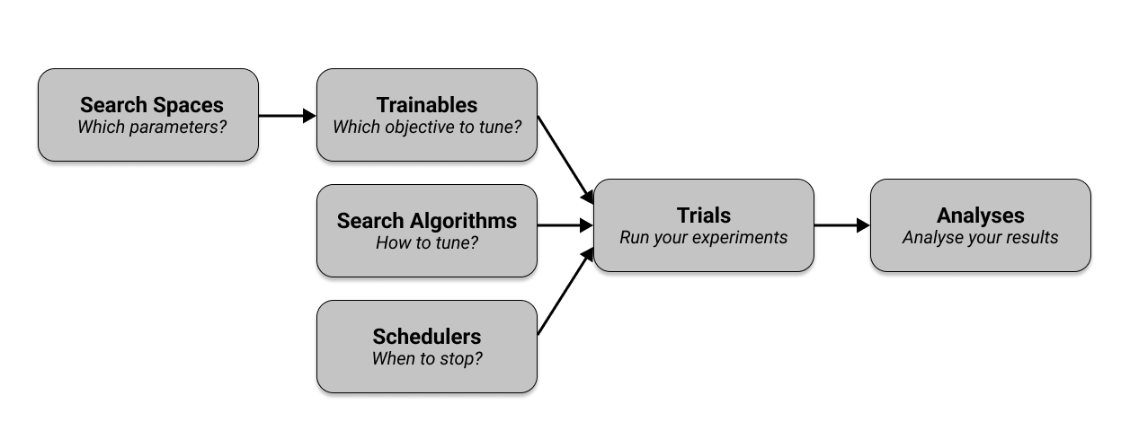
With few python lines you can define, for each of your hyperparameters, the acceptable range. You can then configure a search algorithm to explore the combinations (not just random and grid) and also schedulers to say when it is ok to stop. You pass to the framework the function you want to optimize, and it will do many tests searching for the best parameter combination. Looking at the quickstart example, I imagine you can define a set of experiments like this:

# Define a search space.
search_space = {
    "dropout": tune.grid_search([0.001, 0.01, 0.1]),
    "optimizer": tune.choice([ 'adagrad', 'adadelta', 'sgd']),
}

The quickstart is available on this page https://docs.ray.io/en/latest/tune/index.html , and you can see examples for Keras and PyTorch.

Already this sounds good, but looking a bit around I have found this page: Tune distributed experiments. Ray provides commands to deploy a cluster where you run in parralel your experiments, collect the results, and handles also failures. There are examples for AWS.

Seems really awsome.

Last week I tried to learn more about LSTM, and I was asking myself if there are some rules to choose the hyperparameters. Well, not really rules but al teast some hints: I tried searching for “tuning lstm”, “lstm sizing”, etc and I did not find anything promising. Finally I have found this article:

R.R. Rajalaxmi, L.V. Narasimha Prasad, B. Janakiramaiah, C.S. Pavankumar, N. Neelima, and V.E. Sathishkumar. 2022. Optimizing Hyperparameters and Performance Analysis of LSTM Model in Detecting Fake News on Social media. ACM Trans. Asian Low-Resour. Lang. Inf. Process. Just Accepted (January 2022). https://doi.org/10.1145/3511897

I discovered that some fake news dataset exists, and some researcher are trying to distinguish fake news from true ones, using many different models, not just neural networks.

The ISOT dataset is composed of 21’417 true news and 23’481 fake news. The LIAR dataset instead classifies news in more categories: true, false, mostly true, half true, barely true and pants fire. LIAR is just 6’058 news in total; actually this is the size reported on the paper, on LIAR site the size seems the double – maybe because the dataset comes already divided into train test and validation items.

I was curious to know what a “pants on fire” fake news looks like, here is one:

Wisconsin sold fresh water to California, helping that states dairy industry, and lost a bunch of jobs (and) a bunch of farmland.

LIAR dataset

Ok now I have an idea 🙂

The paper’s authors have built an LSTM model to predict if a news is fake or real; there are no details, I suppose the time factor here is the word position in the phrase, but it is just my guess. Their problem was to pick the right combination of hyperparameters to use, in order to obtain the most accurate model.

To clarify here are some examples

Number of neurons: from 64 to 512

Drop-out rate: from 0.1 to 0.9

Which optimizer to use: adagrad, adadelta, sgd…

I have already found the drop-out rate in other papers: it selects a percentage of neurons to ignore during the training. You may want to do this to prevent the model to overfit the training data: turning randomly off some of your network in the end allows building a less fragile model.

Finally selecting the good hyperparameters combination was just done with grid search and random search. With grid search you just tabulate a long list of possible combination, you take your time to train a model in that case and then compare the results choosing the best one. I did this already many times in a naive way.

With random search insteand, you randomly generate the combinations to be tested. Accoridng to the authors this aproach works in general better.

So in the end I did not find the hints I was looking for, I just come to a new wikipedia page where some more smart methods are also listed: https://en.wikipedia.org/wiki/Hyperparameter_optimization. Maybe the next time I will explore some of them, or I will have a look at the anova method used in the big paper on selecting LSTM architecture: but this one seems requesting a lot of statistics knowledge I don’t have.

Reading just one article on this subject was really not enough for me to undersand. There are still many points not clear and I decided to spend more time on LSTM: read another article, and also search on internet more high level explanations.

I have read the other article proposed by wikipedia on the subject:

Learning to Forget: Continual Prediction with LSTM. Techinical report IDSIA-01-99, January 1999. Felix A. Gers, Jurgen Schmidhuber, Fred Cummins.

The article is from 1999, and it describes why they introduced in the LSTM model the Forget Gate, and explain how this change made the model much more powerful. The reasoning is that, in a recurrent neural network, the output error has to be back-propageted to tune the weights: this becomes a problem considering how the state is memorized.

The cell state in the picture is just a delay, the value at time t will be used at time t+1: if it is updated at each step if will eventually see its value explode due to the sum of errors to track from the beginning of the time. Also the task you have to solve may not require to remember everithing, ad it is legitimate at some point to forget what has happened before. When I have to decide to turn left or right, it has no importance to remember if yesterday a the same time I was turning left, it only matters what I am doing on the current trip, not yesteday’s trip.

This is much more clear considering the benchmark they have chosen, the Embedded Reber Grammar (see this explanation https://cnl.salk.edu/~schraudo/teach/NNcourse/reber.html)

So each message in this grammar can start with BT or BP. If it starts with BT it has to finish with TE, if it starts with BP it has to end with PE. The machine learning model has then to be able to remember this information until the end of the string, which has a variable length, because as you can see in the other blocks of the grammar there are loops. Then as you can see the same grammar block is repeated in the top and bottom branch, but still contains loops, so it is needed to remember what happened in the previous inputs. In the paper they explain that, if you generate 8000 strings, there is a big change you will get one string of at least 50 symbols, so the LSTM will need to remember the BP or BT sequence for a lot of time!

The LSTM model with forget gate is not only able to predict the next symbol of the input stream for the embedded reber grammar, but also the even more complex problem of recognizing sequences of ERG messages. They call this problem the Continuous Embedder Reber Grammar CERG, where one ERG strings follows the other without interruptions. The forget gate will learn whent an EGR sequence is complete and a new one has to start, and will reset the memory cell state, in this way the previous message will not have effect on the current phrase.

So at the beginning of the training the forget gate will be in a state that is near to 1, which means keep the memory untouched, and the memory c will be inizialized with 0. At some point during the training, the forget gate will learn the correct combination of input and previous state that must trigger a reset, and in this case the forget gate will give 0, and make the memory start from scratch. The memory has a formula like c_t+1 = … + forget_gate * c_t, so when the forget gate is 0 it clears the memory.

The role of the other gates in the schema, the input and the output gates, is similar. Theirs value goes from 0 to 1 so that, when the value is close to zero, irrelevant noise and input will not reach the cell changing the state.

To make things simple, I have spoken of c_t but actually nothing prevent introducing many c_1t c_2t etc and have many memory cells. This is actually what is done in the paper, where the model to recognize sequences of ERB strings is composed of 4 LSTM each of them having 2 cells c1 and c2.

If you want a more clear an long explanation I sugget to read https://medium.com/analytics-vidhya/lstms-explained-a-complete-technically-accurate-conceptual-guide-with-keras-2a650327e8f2 where all the pieces are introduced step by step, and the usual picture of LSTM element is decomposed and explained.

Another nice article to read is this one http://colah.github.io/posts/2015-08-Understanding-LSTMs/,

Still after all of this I ask myself how this kind of models have to be sized, if there are some hints on how many c cells to use or h elements to consider. I will continue reading to see if I find something interesting.

After reading the short term weather forcast paper, I was curious about the LTSM and I dedided to learn about it. On wikipedia I have found a reference to this article:

LSTM: a search space odyssey. Klaus Greff, Rupesh K. Srivastava, Jan Koutnìk, Bas R. Steunebrink, Jurgen Schmidhuber. DOI: 10.1109/TNNLS.2016.2582924

It was nice to see that all the authors are from an university really close to my home town! The cv of Jurgen Schmidhuber is really impressive too.

Probably was not the best pick as article because it is not really about LSTM inception but it report on an huge experimentation of different variants, reporting and comparing theirs performances. By converse it has been interesting to see how they managed to fairly compare all these variants, and how they did the hyperparameters tuning.

But what are the LSTM neural networks for? Looking at the 3 use cases used to compare variants performance I see:

• recognising 61 different sound humans can pronounce. The used the TIMIT speach corpus

• recognising handwritten text. The IAM Online Handwriting Database contains hadwritten vector images and the ascii text corresponding to the picture. It is not just a picture as it contains also information on when the pen has been lifted.

• J. S. Bach Chorales, the machine learning model has to learn how harmonies are created. (https://axon.cs.byu.edu/Dan/673/papers/allan.pdf)

So all tasks where time evolution is very important.

The LSTM block itself it is really complicated! First of all there is not just input and output , there are four different input types: block input, plain input, forget gate input, and output gate input. These are taking as input not only the current input, but also the output at t-1. Internally a cell value c is computed and propagated with time delay to the forget gate and to the input gate, and without delay to the output gate; these connections are called peepholes. Finally there is an output block. Sorry, complex and difficult to describe.

The idea is that a memory cell maintains a state over time, and nonlinear gates regulates how information flow into and out of the cell. I reproduce here a similar picture to the one in the article to give an idea, but as the article is available on arxiv it is much better to check the original one directly at page 2.

In formulas:

z_t = nonlin(w_z x_t + r_z y_t-1 +b_z)

i_t = nonlin(w_i x_t + r_i y_t-1 + dot_product(p_i, c_t-1) +b_i)

f_t = nonlin(w_f x_t r_f y_t-1 + dot_product(p_f,c_t-1) + b_f)

c_t = dot_product(z_t, i_t) + dot_product(c_t-1, f_t)

o_t = nonlin( w_o x_t +r_o y_t-1 + dot_product(p_o, c_t) +b_o)

y_t = dot_product(nonlin(c_t) , o_t)

Where w and r are matrices of coefficents; b and p are real coefficients. So complex!

Forget gate is there to let the network learn when to reset itself; my understanding, concerning the handwritten example, the network can learn when a character is completed and a new one is starting, for instance when the text is written in italics. The peephole connextions were introduced to improve learning precise timings.

With a so complex schema it is clear that you can make many small changes to it, and question if that is an improvement or not. That is precisely the scope of the article: they compared the original model with 7 variants.

Since each variant had different schemas and different hyper-parameters, they had firt of all to identify the good seetting for each model and for each set of training data: an huge work but needed to ensure that you compare the best possible results that you can achieve with each model.

The variants compared are: no input gate (always =1), forget gate always 1, output gate always 1, no input activation formula (z(x) = x), no output activation formula (h(c_t) = c_t), coupling input and forget gate together f_t = 1 – i_t, removing peepholes, and full gate recurrence (many more coefficients to feed back in input values of i, f and o at t-1)

Often these changes are not so important, after the training the different networks reach more or less the same performances. This is not true if you remove the output activation function or the forget gate. So from the results those 2 components are very important. Coupling input and forget gates together does not hurt perfomances but reduces the parameters to learn, so seems a good idea to try it. The same for removing the peepholes. Notice also that the very complex full gate recurrence does not bring advantages.

Another interesting part of the article is about how they have tuned the hyper-parameters such as learning rate, momentum, adding gaussian input noise… They refer to the fANOVA framework, and it has let them taking some conlusion on how to tune these parameters.

The learning rate is the most important parameter, start with an high value and decrease it until performance stops increasing. Smaller values will not do better. Adding gaussian noise to the inputs was not useful and they have found that it is not requirend to invest much time in tuning the momentum, as it does not improve significatively the performance.

They also worked on understanding the influence of one hyperparameter on the other, and luckily they seems quite intependent so they can be tuned individually.

Reading some papers I frequently see these kinds of graphs. Since it’s long time I completed my studies, I have forgotten how to use them, and I need a refresh. Here you see one ROC curve taken from Machine Learning-based Short-term Rainfall Prediction from Sky Data. https://doi.org/10.1145/3502731

As usual, a quick look at wikipedia always helps: https://en.wikipedia.org/wiki/Receiver_operating_characteristic. There is a long list of indicator and a long discussion about other ways of selecting a model, a bit too compliaced to digest during a Saturday morning, but here are the key points.

Main assumption: you machine learning model answers a binary question, is there a dog in the picture, or will it rain in 30 minutes. In this context you will have a test set where you have input values and the correct classification label: int this picture there is a dog, in this one no (don’t care if there is a parrot).

I assume that, if your model need to classify pictures betwee dog, cats and parrots, you can end up having one ROC diagram for each class: this picture contains a dog, vs this picture contains a cat or a parrot.

I am pretty sure that, if you have many more classes, you end up with too many curves and this method is not useful anymore.

But to come back to the binary question, you have 4 possible situation for each sample

• the answer is yes and the ML model has found yes: True Positive (TP)
• the answer is no and the ML model has found yes: False Positive (FP)
• the answer is yes and the ML model has found no: False Negative (FN)
• the answer is no and the ML model has found no: True Negative (TN)

This makes things simple to understand, but for me it hides a par of the reasoning: usually ML models depends on parameters, for instance a threshold ML(x,y,z…) so the answer the model can give is a function of these parameters. So TP, FP… are actually TP(x,y,z..), FP(x,y,z..)…

So if you have only one parameter, say t for threshold, you have TP(t), FP(t), etc. As usual you can decide to plot these curves and try to guess the better threshold.

The ROC method tells you to plot together on a cartesian plan these 2 functions

FPR(t) = FP(t)/(FP(t)+TN(t)) fall-out or false positive rate

TPR(t) = TP(t)/(TP(t)+FN(t)) sensitivity, recall, hit-rate or true positive rate

So there are too many names for the same functions, this complicates the things when you read an article.

My conclusion is, if you have many parameters, that you just have to plot on the diagram a family of functions, and then chose the better parameters value to use it in your classification problem. But how do you choose them?

Check this picture on wikipedia: https://en.wikipedia.org/wiki/Receiver_operating_characteristic#/media/File:Roc_curve.svg

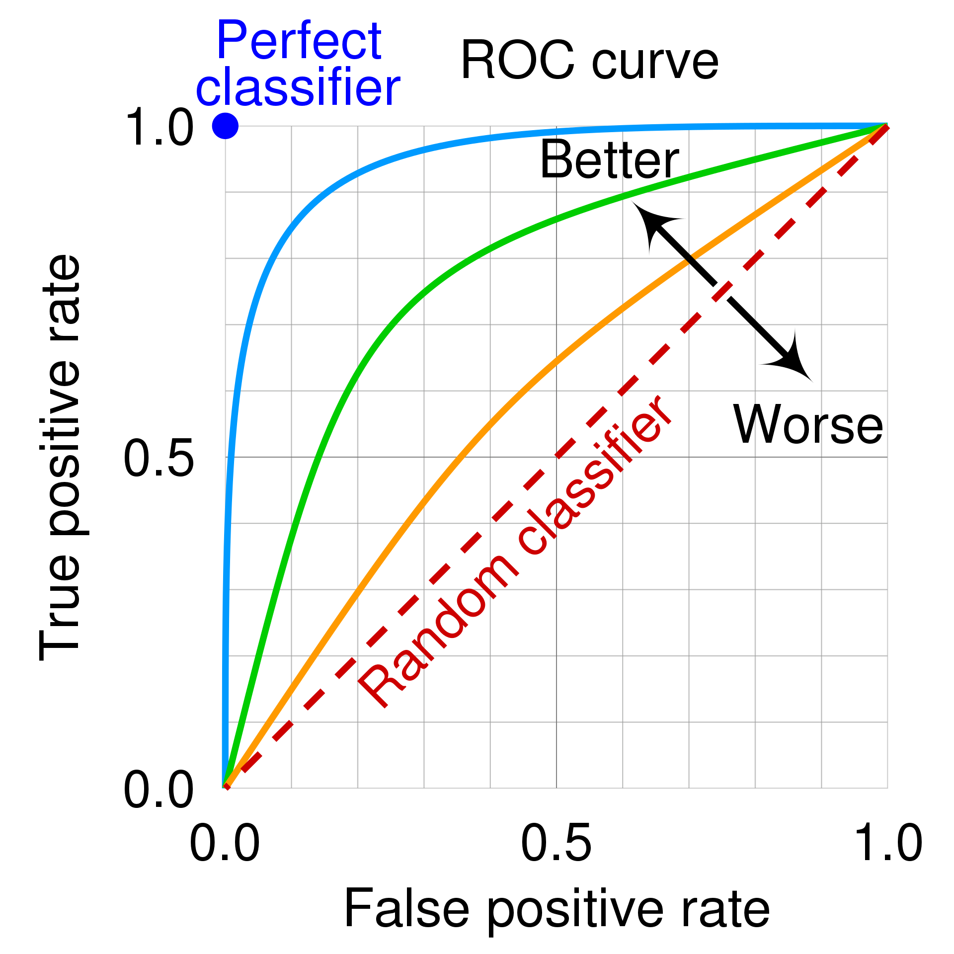
So the upper left corner is the perfect classfier, that is one that has true positive rate of 1: all yes prediction match perfectly the test data, and it has no false positive at all.

My guess is then that you just have to pick the point on your ROC curve that is more close to it and use those parameters.

In the pages I have seen it is always said that the diagonal is the response of a binary random variable: if your ROC curve is close to it, your model is as powerful as flipping one coin and say yes when you see the head, just useless. Also if your model is very bad, just replace yes with now, and you will have a better model (a test that always find that you don’t have covid, and never makes false predictions, would be indeed useful if you want to know if you have the covid).

So what was bothering me of many ROC curves plotted, like the one at the beginning of the page, is that there are no parameter values on the line, and this made me not understand how to actually use them.

This week I have found a nice article:

Fu Jie Tey, Tin-Yu Wu, and Jiann-Liang Chen. 2022. Machine Learning-based Short-term Rainfall Prediction from Sky Data. ACM Trans. Knowl. Discov. Data 16, 6, Article 102 (September 2022), 18 pages. https://doi.org/10.1145/3502731

I enjoyed reading it for various reasons. First of all, it gently introduces some terms and provides many pictures that let you familiarize with the needed concepts. We can guess the meaning of high accuracy, high precision, and recall rate, but it is much better to see the formulas that define them. This is concentrated in a couple of pages, it is a good reference. For instance, accuracy is defined as (# of true positive+true negative predictions)/(all predictions), and precision is just (# of true positive prediction)/(# of true or false positive predictions). Having these 2 pages greatly simplifies interpreting the results presented.

Then it describes how sky data has been acquired. They have deployed some Raspberry-pi modules, taking sky pictures, and also some Arduino-based weather sensors collecting temperature, UV rays, humidity, etc. They describe some difficulties encountered, and some workarounds used, for instance why they have chosen a particular angle when taking sky pictures.

For short-term prediction they mean answering the question: will it rain within 30 minutes? The purpose of the study was to see if a machine learning model, based on sky pictures and some other measures can be accurate enough. Usually, weather forecasts are made using complex mathematical models, on big computers, and their approach requires much less resources.

Their machine learning model is composed of a ResNet-152 convolutional neural network followed by a Long short-term memory recurrent neural network. It has been trained with about 60’000 images and has a recall of 87% on predicting rain absence and 81% on predicting rain.

This week I have decided to read an article about Neural Network interpretation: deep neural networks are made with many layer or many to many connected units, each having many parameters. Once trained they work well but the parameters are too many to understand what they mean, and we have to trust them as black boxes.

As humans we would like instead to have decision trees that we can review, to understand how the decision has been taken. The article I have read was about using neural networks to tune decision rules. You start the training with some expert-defined rules and after the training you get the same rules with better tuned parameters. So the expert can review them and see if they make sense.

The full reference to the article is: Xiaoyu Chen, Yingyan Zeng, Sungku Kang, and Ran Jin. 2022. INN: An Interpretable Neural Network for AI Incubation in Manufacturing. ACM Trans. Intell. Syst. Technol. 13, 5, Article 85 (June 2022), 23 pages. https://doi.org/10.1145/3519313

The idea is that human experts study a problem and are already able to provide some rules to classify the outcome of an experiment. The threshoulds that they set-up are probably sub optimal and they can be improved by some data driven algorithms. The paper refers to the case of crystal growth manufacturing: the expert have already identified some important parameters, such has heater power or pull speed, and have provided an initial model. The model is expressed in term of rules like if x>5 and y<3 or i>6 and j>9 then the crystal is defective (the paper does not provide real rule examples).

What is proposed it to apply a process that translate the rules into a neural network. The particularity is that the layers are not fully connected, but in some layers connections are made just where the input variables are related by model rules. In their case the proposal is to use 4 layers, some rules are provided to help applying the method to different cases.

Once the network is configured, a classical training algorithms can be used
to tune it, and obtain better thresholds in the rules. Notice that they propose
to use a special activation function, called Ca-Sigmoid, to allow incorporating
thresholds in the neural network; this just for the input layer.

Of course the limitation is that the learning process will not learn new rules, it will only optimize the existing ones.

I would like to learn more about machine learning, and I recently came across an interesting ACM journal: Transactions on Intelligent Systems and Technology.

The latest issue (https://dl.acm.org/toc/tist/2022/13/5) contains many papers on federated learning. I have decided to take some notes, not to forget about them. Luckily you can download many of these papers for free if you are interested.

First of all, what is federated learning? Usually, you have a set of input data, classified, and you apply an algorithm to train a model. For instance, you can train a neural network with this data. 

This setting implies that one single entity has access to all the training data, but sometimes this is not possible. For instance, the law can forbid sharing patient data across different hospitals. Also, some counties have laws prohibiting to export personal information outside theirs territory, or protecting consumers’ privacy.

So it is not possible to concentrate all the data in a single place to train a global high-quality model. Models trained just with local data can be less effective, and it is worth finding a way to overcome this limitation.

The approach described in these articles still requires a central coordinator, but it also requires each entity holding the training data to perform model training. From time to time the model parameters are sent from the local entities to the central coordinator. This one updates a global model and sends back the new averaged parameters to each participant. The process is repeated again and again until the training is completed.

Notice that in this way the entities share just parameters and not personal information, overcoming law restrictions. 

Some authors report that federated learning has been originally proposed by Google for the use case of Gboard query suggestion (https://arxiv.org/abs/1610.02527), but I did not read this article.

The first paper I read is: Dimitris Stripelis, Paul M. Thompson, and José Luis Ambite. 2022. Semi-Synchronous Federated Learning for Energy-Efficient Training and Accelerated Convergence in Cross-Silo Settings. ACM Trans. Intell. Syst. Technol. 13, 5, Article 78 (October 2022), 29 pages. https://doi.org/10.1145/3524885. It describes synchronous and asynchronous approaches to Federated Learning, and proposes a new algorithm to share model parameters across the participants.

From what I have got, with synchronous learning, each participant trains its model for a fixed number of ephocs and sends an update to the coordinator. When the coordinator has all the updates, it changes the global model that is sent back to the participants. The process then repeats.

If the participants are different, some fast and some slow, the training proceeds slowly and the more powerful sites are underused.

With asynchronous learning, each participant works at their own pace and there is more communication with the central coordinator, each time an epoch is completed. More communication means more energy consumed, and the paper gives some insight into this problem. Another problem is that slower participants continue training on an old model, while the coordinator has a better version, computed using faster participants’ updates.

With their proposal, the training proceeds until a fixed time limit and the updated models are computed and shared across all participants. The paper explains also how the parameters are averaged.

Another interesting point I have learned is the IID/non-IID assumption. IID stands for Independent and Identically Distributed. If all the participants have IID data, it makes much sense to train a model with all of them. If this is not the case, and one participant is different, this can affect the model convergence.

Another interesting paper is: Trung Kien Dang, Xiang Lan, Jianshu Weng, and Mengling Feng. 2022. Federated Learning for Electronic Health Records. ACM Trans. Intell. Syst. Technol. 13, 5, Article 72 (October 2022), 17 pages. https://doi.org/10.1145/3514500.

It provides a survey of existing applications of Federated Learning on Electronic Health Records, to predict in-hospital mortality and acute kidney injury in intensive care units.

Different algorithms are compared, and one can get references and understand a few of their performances. It also describes CIIL cyclic institutional increment learning: a setting where each party trains a model with its data and passes its parameters to the next hospital. The Federated learning approach, with a central entity assembling a common model, outperforms CIIL approach.   

A few paragraphs above I was writing that it is fine to share model parameters, as they do not contain personal information. But is this really true? Can the central server guess personal information from parameter updates? Xue Jiang, Xuebing Zhou, and Jens Grossklags. 2022. SignDS-FL: Local Differentially Private Federated Learning with Sign-based Dimension Selection. ACM Trans. Intell. Syst. Technol. 13, 5, Article 74 (October 2022), 22 pages. https://doi.org/10.1145/3517820 gives some insight on this point.

The idea is to trade model accuracy with privacy: the model update will not be accurate as it could be and will convey only part of the information. The global model will converge more slowly. 

You can use a random variable to decide which model dimensions you want to share with the central coordinator, and at each update just send these instead of all the updates. In the paper, just k of the smallest or largest model parameters are shared.

The last paper I have read so far is: Bixiao Zeng, Xiaodong Yang, Yiqiang Chen, Hanchao Yu, and Yingwei Zhang. 2022. CLC: A Consensus-based Label Correction Approach in Federated Learning. ACM Trans. Intell. Syst. Technol. 13, 5, Article 75 (October 2022), 23 pages. https://doi.org/10.1145/3519311

Not all participants will have the same ability in assigning correctly the labels to training data. Additionally, with Federated Learning, these samples will not be available to other parties, due to privacy restrictions, so it is not feasible to review them centrally before training the model.

Some of these samples may just be errors, but just removing them may also prevent the model to learn new patterns. Anyway using them early during the training can slow down the learning process or lead to model overfitting.

The method proposed in the article keeps some samples outside the training set during the initial learning epochs. Some thresholds are computed and used later to decide whether to admit the samples in later stages or even correct the label assigned to them.