Giovanni Bricconi

Christmas holidays and the flu have not been propitious to continue my training, but at least I finished watching the video

Machine Learning Algorithms in 7 Days By Shovon Sengupta

Video link

In this post I will just describe what is the content of the remaining chapters, so that who is interested can have a look to the video or to the examples. I believe the examples are very good, showing the good direction when trying something new; they are available on git-hub for free https://github.com/PacktPublishing/Machine-Learning-Algorithms-in-7-Days

The training contains also the following subjects:

• Decision tree
• Random forest
• K-means algorithm
• K-nearest neighbors
• Naive Bayes
• ARIMA time series analysis

The samples show how to use locally Jupyter notebooks with scikit-learn package to train the models

The decision tree chapter describes the concept of purity measure: a new split in the tree will be introduced if it helps classifying better the training examples. For instance the Gini index can be used for categorical variables, but also statistic tests like the chi-square. For numeric variables the F-test can be used. Ideally each terminal node in a tree should output a single category. The video introduces also very quickly the concept of pruning: it is necessary to reduce the number of splits to avoid overfitting. Given the pruning strategy names you can dig further on internet, as the description is too quick. Decision trees have the advantage of being easy to interpret, but they can be unstable to small input changes.

The random forest chapter describes an incremental approach built on top of decision trees. Multiple decision trees are generated selecting different input features: the final classification/prediction can be obtained averaging on the results or choosing the most voted class (softmax) from all the trees in the forest. The video does not speak at all of XGBoost, the algorithm I described some time ago.

The K-Means chapter describes this unsupervised learning algorithm. Using a distance measure some K points (cluster centroids) are chosen, iteratively updating theirs position so that they partition as best as possible the input data. Being based on distance, it is important to normalize the input data, so that one dimension does not take much more importance than the others: if one dimension ranges from 1 to 100 and the other from 1 to 10, it is clear that the squared error is biased. Also you need to deal with categorical data, maybe doing 1 hot encoding. The number of centroids K is a very important parameter for this algorithm, the video describes some methods to find a good value for it.

The KNN (K-nearest neighbors) chapter introduces the concept of finding the closest samples to a point, and speaks about K-D tree and Ball tree algorithms to find the neighbors more efficiently than with brute force. The nearest neighbors found will be used to classify or predict the value for the input point.

Naive Bayes, often used for text classification, is quite effective to perform binary or multi-class classification. Each training sample will have many attribute dimensions, the assumption here is that each attribute value is not correlated with the other dimensions. This is needed to apply the Bayes formula, of course will not be true but applying this simplification still allows to obtain interesting results. This is the example used to explain the concept: you want to predict if a mail is or not spam; of this mail you know the content, the words. You also have a classified mail corpus, where you know if a mails is spam or not and which words were present. The algorithm uses statistics on word count to calculate the probability of a new mail being spam. of course a mail containing the word lottery will probably contain also the word prize, but with naive Bayes you won’t take this into account and just look at prize and lottery distribution. There are many types of naive Bayes algorithm: Gaussian for continuous data, multinomial, and Bernoulli if all features are independent and boolean.

The final Arima chapter, describes how to deal with time series. In this case the input sequence can present a trend and a seasonality, and you want to predict the next values after the sequence end. You apply some techniques to make stationary the input sequence: remove exponential trends, calculate the difference between successive values, etc. The goal is to find a set of parameter that let the Arima model work well, finally producing a residual error that is white noise. The Arima model usually has 3 parameters: the number of autoregressive terms, the number of non seasonal differences, and the number of moving averages. Applying it seems not trivial, but the results produced by the example are quite impressive.

I continued watching

Machine Learning Algorithms in 7 Days By Shovon Sengupta

Video link

And this time the subject was Logistic Regression; having caught cold did not help studying this week, sob. Here are my notes

This is the sigmoid function 1/(1+e^-x), as you can see it goes from 0 to 1, and at x=0 it’s value is 1/2. This function will be used to classify the inputs to two categories 0 or 1, no or yes. Once trained the model, it will be evaluated with the inputs, and the sigmoid will be computed. If the result is closer to 0 then the category 0 will be chosen, otherwise the category will be 1. So logistic regression can by tried whenever you have a binary classification problem, such as will this customer subscribe a new contract?

With a trick it is be possible to extend it to multiple categories: suppose you want to classify the inputs into 3 categories A,B, and C. You can formulate 3 binary questions: is it A or something else? is it B or something else… You can then train 3 logistic model, and each of them will predict an y value, you will chose the category that has the highest y value as the correct category (softmax).

The actual formulation does not use directly the sigmoid, but a logarithm of probabilities. Let’s be p the category 1 probability, the logit function is defined as ln[p / (1-p) ]. The model that will be trained will obey to this equation:

So you can have as many explanatory variables X as you want. The training process will identify the theta coefficients that minimize the classification error.

As for the linear regression, the training continues presenting a plethora of statistic indexes to judge the trained model: concordance, deviance, Somer’s D, C statistic, divergence, likelihood ratio, Wald chi-square… Luckily the sample code can be used to understand practically what to do in a Jupyter Notebook: https://github.com/PacktPublishing/Machine-Learning-Algorithms-in-7-Days/blob/master/Section%201/Code/MLA_7D_LGR_V2.ipynb

The samples contains examples on:

• Identify categorical variables, and how to generate dummy variables to be used in the training
• How to plot frequence histograms, to explore the data
• How to produce boxplots, to understand data distribution
• Using the describe function to get avg, stddev and quantile distributions
• Using Recursive Feature Elimination, to select only the most relevant explanatory variables
• Using MinMax scalers to prepare the data and how to train the logistic regression model
• Check for multi-collinearity and further reduce the used explanatory variables
• Plot the model’s ROC (receiver operating characteristic)
• Plot a Shap diagram to understand which are the most relevant libraries and how they influence the classifier.

This week I have been suggested to watch this video:

Machine Learning Algorithms in 7 Days

Video link

By Shovon Sengupta

It’s 5 hours and a half video on machine learning algorithms, authored by a principal data scientist at Fidelity Investments. Of course I did not have 5 hours spare time this week to follow it all, I just started watching the first “chapter” on linear regression. Shovon Sengupta made the subject passionating adding a lot of references to statistic tests. Actually the chapter goes so fast that you need to take some extra time searching explanations and definitions to understand better. Luckily there is support material, and you have access to a git report with the Jupyter notebooks used, so you can read them an test them later.

So what is the recipe to cook a linear regression?

• Clean the input data: check for missing data and decide what to do with outliers as the linear regression will be influenced by them. I hope that for outliers there will be another section in the video because in this part it went too quick – but in the sample there is at least one suggestion
• Check for multi-collinearity: this is interesting and well explained. It may happen that some of the input variables (explanatory variables) have a linear correlation between them, so they are not really independent. To make an absurd example you can have two input columns, one in the temperature in Fahrenheit degrees and the other in Celsius degrees. You must not use both of them or the linear regression algorithm may not work well.
• Select the features: you should analyze the explanatory variables to decide which ones to use, those that have more influence on the output variable. The training explains the Ridge and LASSO methods.
• Build the model on some training data
• Validate the model performance on test data.

So, even if it is just a linear regression, to do it well you need to do many not obvious things. Here I list for myself many definitions that are needed to understand the samples provided in the training

R2 explains the proportion of variance explained by the model

So the sum of squared prediction errors divided by the error you have pretending that the model is just the constant average value

You can have a better adjusted R2 index, taking into account the number of samples you have n and the number of input variable you use p:

You use R2 to calculate the variance inflation factor that is just 1/(1-R2) and it is an indicator useful to check if there is multicollienarity. The lower the better

The F statistic to check if there is a good relationship between the predicted output and the chosen explanatory variables. The higher the value the better is the relation.

The Durbin Watson test is instead used to test the presence of autocorrelation:

It will always have a value ranging between 0 and 4. A value of 2.0 indicates there is no autocorrelation detected in the sample. Values from 0 to less than 2 point to positive autocorrelation and values from 2 to 4 means negative autocorrelation. 

DW test statistic values in the range of 1.5 to 2.5 are relatively normal. Values outside this range could, however, be a cause for concern

From <https://www.investopedia.com/terms/d/durbin-watson-statistic.asp>

Another concept to check is the prediction error homoscedasticity: is the error just coming from a normal distribution or does it have an evolution? With the Breusch Pagan test you can check if the error

The last interesting concept is the regularization: the coefficients identified by the regression algorithm can tend to explode, or include variable that cause sample data overfitting. It is important to boost simpler models and this can be done introducing some penalty terms in the loss function

LassO  Least Absolute Shrinkage and Selection Operator,

Ridge

The lasso method has the advantage of removing low importance variables from the model, while the Ridge makes them very small but not zero. See <https://www.datacamp.com/tutorial/tutorial-lasso-ridge-regression> for a nice description.

But concretely how to use all these concepts? Luckily the training points to this git repository, where you have a nice python script that step by steps applies many of these checks on some sample data, and produces many graphs that helps understanding the concepts. https://github.com/PacktPublishing/Machine-Learning-Algorithms-in-7-Days/blob/master/Section%201/Code/MLA_7D_LR_V1.ipynb

Nothing easier than a linear regression? Not at all, if you don’t want just scratch the surface!

Last week I read about the XGBoost library and I wanted to understand more about the theory behind it. I started then reading this referenced article, and I have found a lot of explanations:

Jerome H. Friedman. “Greedy function approximation: A gradient boosting machine..” Ann. Statist. 29 (5) 1189 – 1232, October 2001. https://doi.org/10.1214/aos/1013203451

The document is very long, more than 40 pages, dense of math and statics; something too long to digest in my short weekly spare time. This is what I have learned so far. The goal of this method is to approximate an unknown function given the inputs and outputs collected in the past. This is very general, and requires a Loss function to be defined.

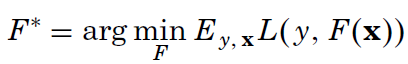
We search for the F* function that minimizes the average loss, given the past input (x is a vector), and y (a scalar output). The article explores three different loss functions; among them the usual square-error and the Huber loss function – something new to me and here is its definition:

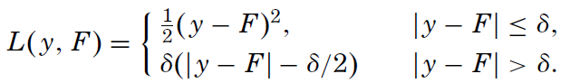
The author has chosen this function because he is looking for an highly robust learning procedure: if the difference between the predicted output and the real one is smaller than delta, it is used, otherwise just the error direction is taken into account. In this way the procedure will discard outliers. Of course, using the Huber loss function, you need to decide the delta value.

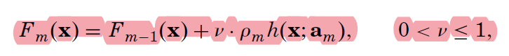
But how do you search for F*? We will not look for whatever function, but we will restrict the search to a function family, regression trees. The single functions will be identified by a parameter set a={a_1,a_2…}. With XGBoost we were adding one new regression tree at each learning step, this comes from the way the gradient boosting searches for F*: additive expansion

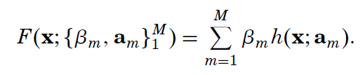
At each leaning step m, a new simple function beta_m*h(x1,…,a_1,…,a_m) is added to the previous approximation: in this way a more and more complex function is built. The prediction will not diverge, as the added function produces positives or negatives values. This method is very powerful! This is the author’s explanation:

Such expansions (2) are at the heart of many function approximation methods such as neural networks [Rumelhart, Hinton, and Williams (1986)], radial basis functions [Powell (1987)], MARS [Friedman (1991)], wavelets [Donoho(1993)] and support vector machines [Vapnik (1995)]. Of special interest here is the case where each of the functions h(x,a_m) is a small regression tree,
such as those produced by CART TM [Breiman, Friedman, Olshen and Stone (1983)]. For a regression tree the parameters a_m are the splitting variables, split locations and the terminal node means of the individual trees.

How do you choose the next beta_m*h(x1,…,a_1,…,a_m)? You chose the best function that minimize the Loss function: with appropriate function this corresponds to calculate a derivative, and find the parameters that makes this value zero, to find its minimum. The article becomes dense of math and statistics, as you have a finite set of inputs, and regression trees are not really function where you can calculate a derivative! I really miss a lot of theory to understand the paper.

The paper describes a generic algorithm that must be adapted to different loss functions to be used.

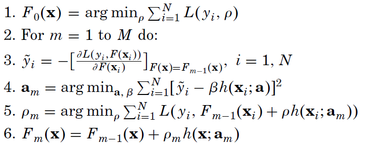
You start from an F_0 initial approximation, at each new step you calculate y~ given the past knowledge. You search then the best h_m that tries to match the optimal gradient descend and you choose the optimal weight rho to add h_m to the additive expansion.

The article continues deriving the correct algorithms to use with different loss functions and the introduces the “regularization”. Practical experience suggest to introduce a learning rate v constant, that is used to scale down the influence of new learned trees.

To apply the algorithm then you will have to choose the good M and v values. The article continues presenting some simulations and suggestion on which loss function to chose and how to choose these parameters. Another important parameter identified is J: the terminal nodes allowed to be in the regression trees. A too low J does not allow to learn complex relations, a too high value opens the door to over-fitting.

When reading the AutoML benchmark I saw that XGBoost was one of the more recommended models: I decided to learn about it and I read this paper:

XGBoost: A Scalable Tree Boosting System. Tianqi Chen, Carlos Guestrin, KDD ’16, August 13-17, 2016, San Francisco, CA, USA https://dl.acm.org/doi/10.1145/2939672.2939785

The article dates 2016, and reports that at that time this algorithm has been successfully used in many competitions obtaining the best placements. Among the 29 challenge winning solutions published at Kaggle’s blog during 2015, 17 solutions used XGBoost. Among these solutions, eight solely used XGBoost to train the model, while most others combined XGBoost with neural nets. A similar situation is reported for the KDD cup in 2015. This algorithm scales up to billion of training samples, and is open source and available on https://github.com/dmlc/xgboost and currently active.

The algorithm consists in finding a tree set: in each tree an internal node consists in a condition on the inputs features, and the leafs consists of real numbers. With a new set of inputs, each tree is evaluated and provides one weight, all the weight are summed to give a final results, that is the classification/prediction searched. Given this structure is easy to understand that it is very easy to parallelize the evaluation, obtaining good performances.

The paper describes many optimization done to make the algorithm fast. It is quite common for input data to be sparse, for instance because one-hot encoding has been used, or because many values are absent. This has been take into account, and the authors reports that the sparsity-aware algorithm runs 50 time faster that the basic version. The input data are prepared, sorting them in ascending order, and dividing inputs in blocks. Choosing the right block size allows to avoid cache misses in data access, and also allows to run the analysis on multiple cores/servers. Prepared data can also be reused many times, avoiding to pay again and again the preparation cost. The data blocks can be compressed and the work divided into reading threads and processing threads: the reading threads read an decompress the blocks, while the processing threads process them. The authors suggest also to shard the input data on multiple disks, to parallelize the access and improve performances. For instance the authors report:

We can find that compression helps to speed up computation by factor of three, and sharding into two disks further gives 2x speedup. For this type of experiment, it is important to use a very large dataset to drain the system file cache for a real out-of-core setting… Our final method is able to process 1.7 billion examples on a single machine

All these details testify the amount of work and interest for this library.

But how this library builds a model from the input data? Let’s first of all introduce some names

n is the number of input samples

m is the number of input features (dimensions)

Each input sample is composed of <x1, x2, … x_m, y> where y is the value to be predicted

i is the index in the n samples

K is the number of trees used to predict y

T is the number of leaves in a tree

w is the weight attached to a leaf

t is the learning iteration

The function that is optimized by this algorithm is

So the difference between the actual and predicted value plus a normalization factor that penalizes the number of nodes used in the trees T and the square of the weights used in the models. This normalization has been added to penalize complex models with high values, and is effective on preventing overfitting.

The algorithm iteratively adds one new tree at each step, choosing the tree that reduces the most the loss function L.

Above you see an approximation that is used in the algorithm: g_i and h_i are the first and second order derivative, and f_t is the tree function that we are looking for at iteration t. Really I do not understand how you can get these derivative, I will have to read the bibliography to understand how it is possible to calculate these values.

After some steps the authors present how to calculate the optimal value for a new tree leaf, and how much a proposed tree will reduce L

Here I_j is the set of input that is selected by the jth leaf in the proposed tree. The algorithm iteratively builds a new tree adding more and more splits, calculates the improvement of each tree and at the end chooses the best tree. To decide the splits the authors introduced a quantile based approach, so the splits are done evenly over data distribution.

The sparse data optimization consists in choosing a default direction in the trees: each time an input is missing you follow that direction. The good direction is decided tree by tree, of course the one that minimizes L

In the end the good tree is chosen enumerating possibilities, and using multiplications and sums: so you can create a good model using a very large set of trees instead of stacking layers and layers of neurons.

I think I have explored enough the hyper-parameters tuning tools: to conclude this series I had a look at Katib because it fits well the environment I can use at work. This time I did not have fun looking at strange algorithms, as Katib is just a shell that allows you to run comfortably optimization tools in Kubernetes. By chance I saw in Google that Katib, or better Kātib, was a writer, scribe, or secretary in the Arabic-speaking world (Wikipedia): indeed the tool keep tracks of optimization results, schedules new executions and provide an UI, a good secretary job.

This paper describes Katib:

A Scalable and Cloud-Native Hyperparameter Tuning System. Johnu George, Ce Gao, Richard Liu, Hou Gang Liu, Yuan Tang, Ramdoot Pydipaty, Amit Kumar Saha. arXiv:2006.02085v2 [cs.DC] 8 Jun 2020

link: https://arxiv.org/abs/2006.02085

The authors are from Cisco, Google, IBM, Caicloud, and Ant Financial Services.

Katib is part of Kubeflow, a Kubernetes platform to industrialize working on machine learning. Katib does not offer you a specific algorithm to optimize parameters, it is instead a shell allowing you to run in a reliable way other tools. From the article introduction you get that: you must be familiar with Kubernetes, you can run it on your laptop but in the end is done to run on a Kubernetes cluster, it is open source, and it is thought also for operation guys.

As it is built on top of Kubernetes, you can have one cluster with many namespaces into it, and segregate each team work into a different namespace. You can leverage Kube role management, to configure the permissions to access these namespaces. Katib provides logging an monitoring to get insight in what it is going on during the simulations.

As many other Kube tools, you configure your experiments with yaml resources. These resources are fetched from some controllers that update theirs states and tries to fulfill what you are asking for. this is the example reported in the paper:

The parallelTrialCount allow to specify how many processes to run in parallel, to limit the resources used by a team. As you can imagine, scalability is not an issues as all works the cloud way. The authors say they used chaos-engineering tools to stress Katib and verify that it is robust enough to be user in real applications.

This is a reporting view on trial results:

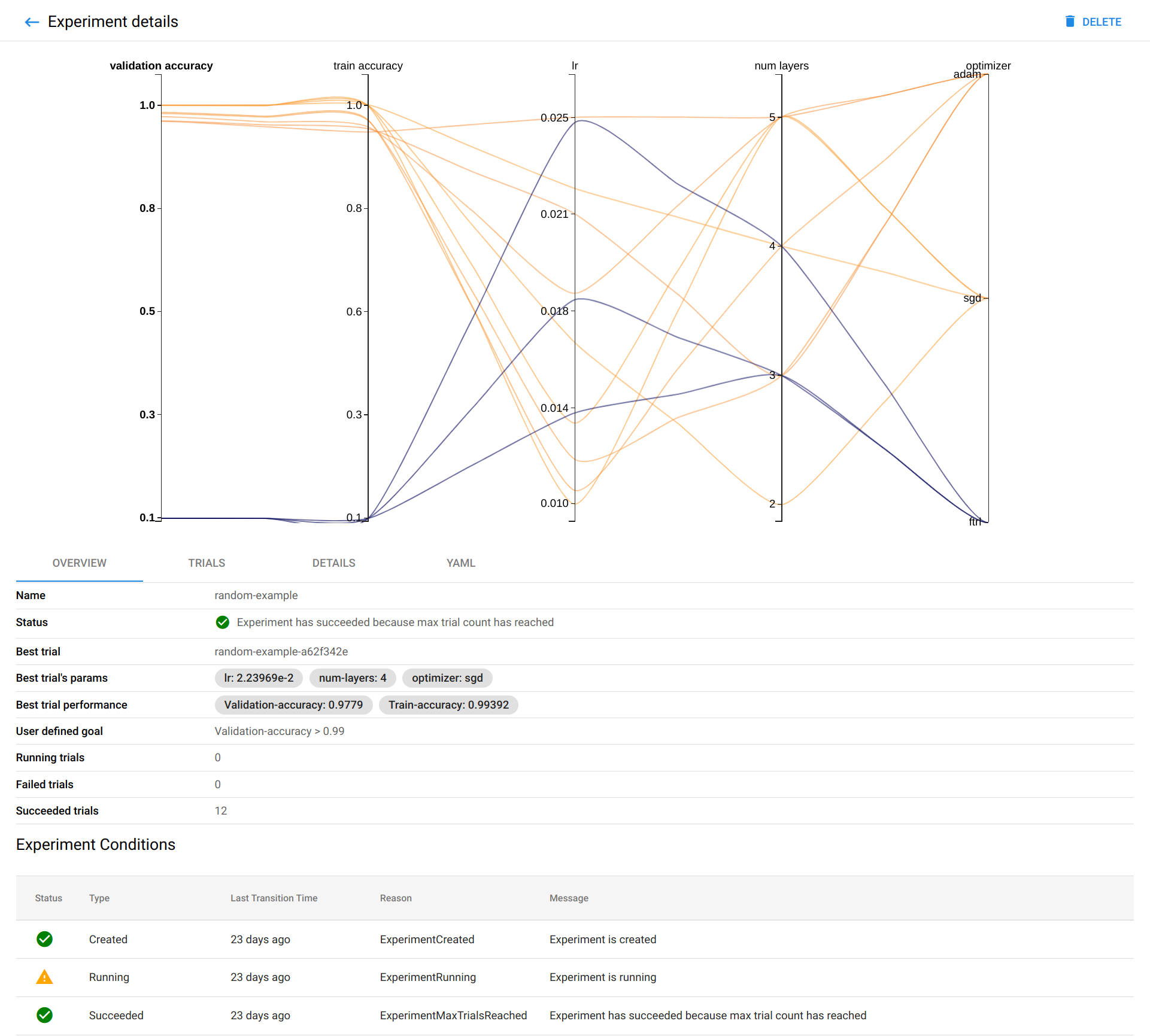
The leftmost axis, called validation accuracy, is the target function to optimize – here the higher the better. Following the orange lines on the other axis you can see which have been the hyper-parameters values that have given the better results. For instance here seems it is better to have the learning rate between 0.01 and 0.018.

And that’s all I had to say.

Some time has passed since I wrote about climate change: I have been busy, but progressed on my solar panels project. You will see that this requires a lot of time here in France.

Photo by Bill Mead on Unsplash

In April this year, I started asking myself if I could put solar panels on my roof and what benefits I can expect. I could just switch to a contract that guarantees green electricity, but I liked the idea of being part of the energy transition. I like also the idea of being more independent from electric companies: now that there is a war in Ukraine, and all the energy prices explose, I feel right.

But what should you do to have solar panels on your roof? It is not an easy task where you choose a module, and you install it yourself. You need the right stuff to fix them, the right cables, the inverter, fill many administrative papers… too many things to know. So I asked for a quote to three different big companies. As I am a stranger here in France and I don’t have many contacts, I preferred to avoid asking quotes to small shops.

I got a wide range of prices: 8000 euros, 10000 euros and 13000 euros for the same installation of 3 kw peak power. I checked the reputation of the cheapest provider: the customers comments weren’t that good. 5000 euros difference seems to me a bit too much anyway.

The guy of the 10000 offer was really professional and provided me many details on the equipment and the laws. Unfortunately you cannot just choose a provider and do the installation.

I live in a co-property: I own one house, but it is inside a big complex. I need to ask a permission to the administrator to make any changes to the house exterior. When I asked the administrator, they replied that I had to present a project and have it voted to the owners assembly. I asked this in April, and the assembly has been just held this November 17! Seven months delay!

Here in France you have the right to install a plug in the co-property if you need to recharge an electric car, just presenting some documentation. The same for a TV antenna, but if you want to produce your own energy you can’t.
Many speaks of energy transition, climate change, but when you want to act, you realize that it is all so complicated.

Also the incentives the country provide are not that good. For a 3kw installation you will get 1000 euro only, payed in 5 years! If you buy an electric car you get 6000 euro now! Your VAT is reduced to 10% but only if your installation is not above 3kw. If you want to produce more, you pay 20% VAT. Isn’t this a mistake? The more solar energy, the more autonomy from foreign countries.
Also you can sell 1 kw of solar energy to the electric grid, but you will get 0.10 euros. If you look at your bill, you will see the price is about 0.16… and this was before the war beginning.

So a lot of time passed, but I will tell what happened in the owner assembly next time – and then you will understand why I have put the word “ugly” in the title

I wanted to find a tool implementing the TPE algorithm to explore the model hyper-parameter spaces, and after searching a bit I have found the original implementation, but there was no recent activity on it. After some other tries I have found Optuna and the article that introduces it:

Takuya Akiba, Shotaro Sano, Toshihiko Yanase, Takeru Ohta, Masanori
Koyama. 2019. Optuna: A Next-generation Hyperparameter Optimization
Framework. In The 25th ACM SIGKDD Conference on Knowledge Discovery
and Data Mining (KDD ’19), August 4–8, 2019, Anchorage, AK, USA. ACM,
New York, NY, USA, 9 pages. https://doi.org/10.1145/3292500.3330701

The article is quite recent and provides references to other similar tools that can be useful: Spearmint and GPyOpt which use Gaussian Processes, Hyperopt employs tree-structured Parzen estimator (TPE), SMAC uses random forests, Google Vizier Katib
and Tune also support pruning algorithms, Ray Tune.

What makes Optuna special? It’s approach in defining the hyper-parameters space to explore. The example provided by the authors is very clear: they propose to tune a neural network that can have up to 4 layer, and where each layer can have up to 128 units. What is the difficulty here? You will always have a number of neurons for layer 1, but you will have a number of neurons for layer 3 only if layer 2 and layer 3 exists. For instance with Hyperopt you need to use choice constructs to describe this conditional relation and the code is not so easy to read. With Optuna instead you have this approach, called define-by-run:

Using Optuna you define a study (line 20) and you want to optimize it in 100 trials (line 21). The objective function defines which hyper-parameters are pertinent and the loss function. The trial here is the current test instance, at line 5 it is said that the model has up to 4 layers: actually at that point when executing the code Optuna will use the past experiments to decide which is the best candidate value to use. Then, with a simple for loop it is asked to Optuna to get the most promising number of neurons for each layer. It is easy to do so because you do not need to deal with condition, at that point in the code you know that you have x layers and you can just define the parameters needed. The rest of the code is to use the parameters, read the train and test data and compute the model performance.

With Hyperopt instead you have to do something like this:

You can find the complete examples in the paper. It is easy to understand that, with more and more options to explore, a model made with Optuna will be easier to understand and modify.

Optuna has also something more to offer: an efficient pruning algorithm: unpromising trials are abandoned before a complete train/test cycle, freeing resources to explore other configurations. The pruning algorithm used is named Asynchronous Successive Halving(ASHA) and is an extension of Successive Halving. To understand how it works it is better to read the article describing successive halving:

Kevin Jamieson, Ameet Talwalkar. Non-stochastic Best Arm Identification and Hyperparameter Optimization. Proceedings of the 19th International Conference on Artificial Intelligence and Statistics (AISTATS) 2016, Cadiz, Spain.

Here Arm refers to a specific hyper-parameter instance. Intermediate loss functions values are compared between different arms, only half of the arms will survive each time selecting the best ones. In this setting, the question is not if the algorithm will identify the best arm, but how fast it does so relative to a baseline method, as no specific statistic assumptions are made. The plots published in the paper are really encouraging.

Coming back to Optuna, you can choose the algorithm used to select the next candidates parameters: you have TPE and also a mix of TPE and CMA-CS. According to the authors, GPyOpt can obtain better results but it is one order of magnitude slower than Optuna.

Other Optuna advantages are that you can choose the backend used to store the trials performances (for instance use a database), and that it is easy to install it and use it in conjunction with Jupyter and Pandas.

To conclude, you can use Optuna also for tasks not related to neural networks and machine learning: the authors reports that it has bee used to find optimal parameters for RocksDB (which has many many parameters to tune) and ffmpeg configurations for video encoding

While searching for tools implementing the techniques I have recently read (variance analysis and optimized hyper-parameter search) I have found this interesting paper:

L. Ferreira, A. Pilastri, C. M. Martins, P. M. Pires and P. Cortez, “A Comparison of AutoML Tools for Machine Learning, Deep Learning and XGBoost,” 2021 International Joint Conference on Neural Networks (IJCNN), 2021, pp. 1-8, doi: 10.1109/IJCNN52387.2021.9534091.

pdf download

The authors have listed a long set of tools and conducted may experiments to compare recent AutoML solutions. But what is AutoML? The idea is that it is possible to build tools that allow non-experts to make use of machine learning models and techniques without requiring them to become experts in machine learning. Wikipedia

In the paper they compared these tools: Auto-Keras, Auto-PyTorch, Auto-Sklearn, AutoGluon, H2O AutoML, rminer, TPOT and TransmogrifAI. To compare them, they used 12 different OpenML datasets divided in 3 different scenarios General Machine Learning (GML), Deep Learning (DL) and XGBoost(XGB). So 8 tool by 12 models, 96 combinations, for sure there is a big effort behind this study. In the paper you find also a lot of references to other studies and tool descriptions, precious if you want to explore further.

The datasets used to compare the tools are the most downloaded ones from OpenML, and the tools have been used with theirs default parameters, as newbie user would do. The results reported privileges in first place the obtained model performance, and in second place the time spent performing the analysis.

For what concerns general machine learning, the data sets have been divided in binary classification, multi-class and regression tasks. There is not a tool that wins the other in all categories: TransmogrifAI is the best for binary classification, but H2O is very very close. In multi-class categorization AutoGluon is the best but again H2O is very close. Finally for regression there is no much difference between the results. For deep learning models, again H2O is one of the best tool. AutoGluon again wins in one sub-category. In XGB scenarios the the best tools are rminer and H2O.

There is one more interesting point: the models created by these tools have performances close to the best reported in on OpenML, so these tools are definitively something to try.

Given the results I had quickly a look to H2O site, as it appears so often in the top scores. The sample linked here is quite easy to understand.

import h2o
from h2o.automl import H2OAutoML

# Start the H2O cluster (locally)
h2o.init()

# Import a sample binary outcome train/test set into H2O
train = h2o.import_file("https://s3.amazonaws.com/erin-data/higgs/higgs_train_10k.csv")
test = h2o.import_file("https://s3.amazonaws.com/erin-data/higgs/higgs_test_5k.csv")

# Identify predictors and response
x = train.columns
y = "response"
x.remove(y)

# For binary classification, response should be a factor
train[y] = train[y].asfactor()
test[y] = test[y].asfactor()

# Run AutoML for 20 base models
aml = H2OAutoML(max_models=20, seed=1)
aml.train(x=x, y=y, training_frame=train)

# View the AutoML Leaderboard
lb = aml.leaderboard
lb.head(rows=lb.nrows)  # Print all rows instead of default (10 rows)

# model_id                                                  auc    logloss    mean_per_class_error      rmse       mse
# ---------------------------------------------------  --------  ---------  ----------------------  --------  --------
# StackedEnsemble_AllModels_AutoML_20181212_105540     0.789801   0.551109                0.333174  0.43211   0.186719
# StackedEnsemble_BestOfFamily_AutoML_20181212_105540  0.788425   0.552145                0.323192  0.432625  0.187165
# XGBoost_1_AutoML_20181212_105540                     0.784651   0.55753                 0.325471  0.434949  0.189181
...

I have copied the example from this page: https://docs.h2o.ai/h2o/latest-stable/h2o-docs/automl.html#code-examples. So with few lines of code you can define how many model to test and obtain indications on which one to pick. This page is quite long and provides many information; for instance you see wich models H2O is able to investigate: three pre-specified XGBoost GBM (Gradient Boosting Machine) models, a fixed grid of GLMs, a default Random Forest (DRF), five pre-specified H2O GBMs, a near-default Deep Neural Net, an Extremely Randomized Forest (XRT), a random grid of XGBoost GBMs, a random grid of H2O GBMs, and a random grid of Deep Neural Nets. You see also the list of hyper-parameters that will be searched with grid search.

Last time I read Hutter’s article on assessing parameter importance: it is interesting, but how to apply it without some tooling? Well, at the article’s bottom there was a link to a tool, but the article was dated 2014 so it could have been abandoned. I am lucky, after searching a bit I have found the new location:

http://automl.github.io/fanova/

So the tool is now part of a bigger initiative https://www.automl.org/ whose goals are:

• making machine learning more accessible
• improving efficiency of machine learning systems
• accelerating research and AI application development

This initiative is led by Prof. Frank Hutter (University of Freiburg), and Prof. Marius Lindauer (the Leibniz University of Hannover).

The last git commit dates 2020, but the documentation seems good and the tool easy to use. This is the f-ANOVA quick start guide.

To analyze hyper-parameters importance you need to prepare a couple of files, one containing the parameter values, and one containing the loss-function result after the testing.

>>> from fanova import fANOVA
>>> import csv
>>> X = np.loadtxt('./online_lda_features.csv', delimiter=",")
>>> Y = np.loadtxt('./online_lda_responses.csv', delimiter=",")
>>> f = fANOVA(X,Y)
>>> f.quantify_importance((0, ))
 0.075414122571199116

You provide the inputs and with the last method you get the importance of the 1st parameter: it is a little value other parameters must be more important for this model. You simply do the same with the other parameters and decide which parameter should be investigated the most. You can also use the get_most_important_pairwise_marginals method to understand which parameters interact the most. The package provides also some visualization function that allows showing beautiful graphs like this one:

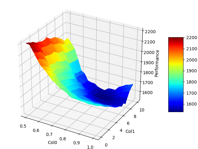
The f-ANOVA starter page explains briefly how to proceed and interpret the results.

The code is available on GitHub: https://github.com/automl/fanova/tree/master/examples/example_data/online_lda