Giovanni Bricconi

Looking for new ideas I have found an interesting ACM Journal, CSUR ACM Computing Surveys, which publishes surveys helpful to get introduced to new subjects; a place to have a look at from times to time. Browsing the latest issue I have found this article:

Rudresh Dwivedi, Devam Dave, Het Naik, Smiti Singhal, Rana Omer, Pankesh Patel, Bin Qian, Zhenyu Wen,
Tejal Shah, Graham Morgan, and Rajiv Ranjan. 2023. Explainable AI (XAI): Core Ideas, Techniques, and Solutions.
ACM Comput. Surv. 55, 9, Article 194 (January 2023), 33 pages.
https://doi.org/10.1145/3561048

It’s quite long, 30 pages, and it describes many techniques and tools useful to understand ML models; for instance LIME and SHAP graphs are explained, with some examples, and this will help me better understanding many other papers.

XAI is helpful in two contexts: when you are developing a model it will help you understanding if it is precise enough and if it can be used as intended, when the model is deployed, XAI will help you explaining why a decision has been taken. The understanding consists in identifying the most important features, theirs relations, the presence of bias in the training data etc.

There are many XAI techniques, they can be divided in many ways. You have model agnostic and model specific techniques, if they target or not a specific model. You have global interpretation or local interpretation depending if the technique tries to explain in general what the model is doing, or it is limited to explain why a decision has been taken for a specific input.

The paper has many sections, the ones I liked the most are “Feature Importance” and “Example-Based Techniques”, but there are other sections about tools for model explainability (Arize AI, AIF360, AIX360, InterpretML, Amazon SageMaker, and Fairlearn) and distributed learning.

To understand features, you can use the Permutation importance technique: it is computational expensive but it’s output is a nice table with a number for each feature, the higher the value the more important the feature is. You have also PDP Partial Dependence Plots, whose output is a graph. On the x-axis one feature, and a line with the predicted value, around the line a confidence area. This technique analyzes a feature at the time, and does not take into account correlations.

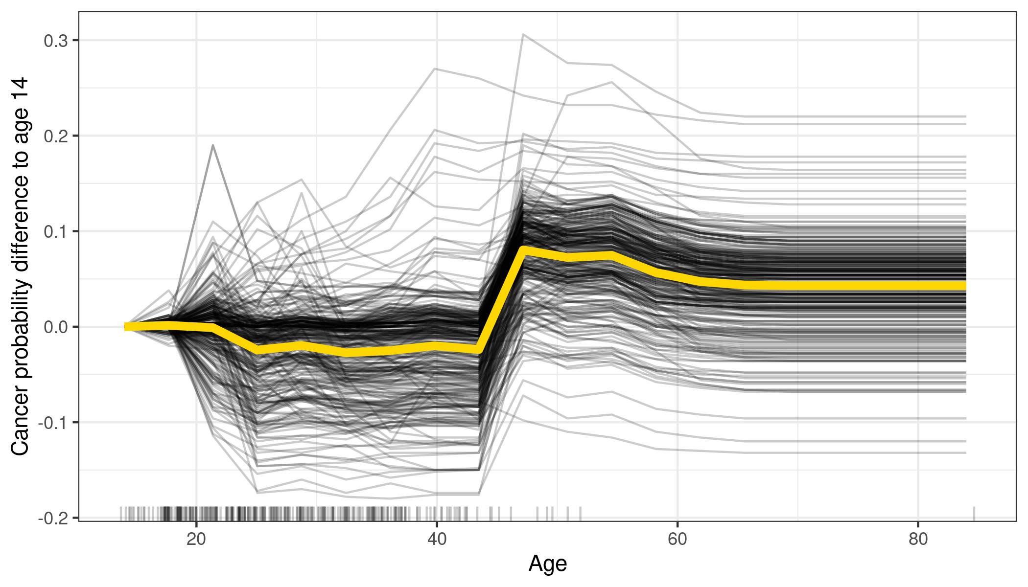
ICE Individual Conditional Expectation plots are very similar to PDP, instead of seeing a gray area around the line, you will see many lines showing what is happening for various instances. Of course if you plot too many instances you will have something difficult or impossible to read, but it is more easier that interpret than the gray area in PDPs.

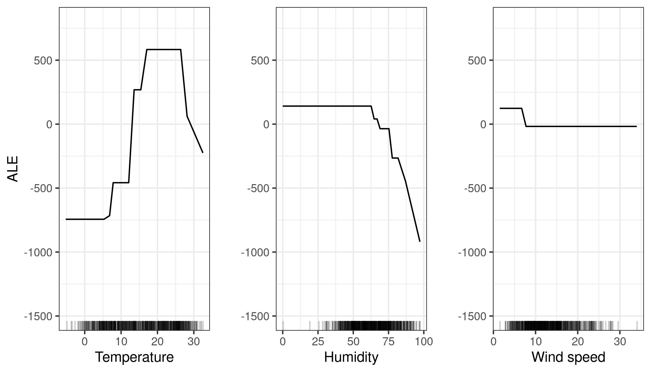
ALE Accumulated Local Effects are another way to visualize features importance: the authors do not explain much about them, they just say that the work also well if features are correlated. Below you see an example about bike rentals, it is easy to understand when a feature becomes important: when is raining (high humidity) people do not want to rent a bike.

Moving to local interpretation, you have the LIME Local Interpretable Model-Agnostic Explanations technique: a sample input is perturbed and the impact on the prediction is captured. With images it is really easy to understand which elements the model is taking into account to make a prediction

Lime can work in other contexts than images, showing which feature values are increasing (or decreasing) the prediction

Another great tool to visualize feature importance is SHAP:

Here features are sorted by theirs impact, Feature 1 has more impact than Feature 0. When the bar is red painted, that value will make the prediction increase, when it is blue it will make the prediction decrease. Shap output can also be represented in this way:

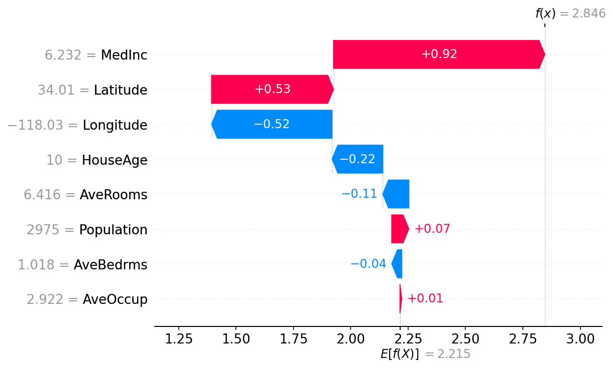
Here you see how each feature has contributed to the final result, starting from the average model prediction. AveOccup and AveBedrms have nearly no impact, Populations contributes to the house price a bit more, AveRooms decrease it, etc until MedInc that contributed the most, and the final prediction is 2.846. Each observation will have its own SHAP diagram.

Another interesting question you can ask is “what is the minimum change of a feature that can make the model prediction change?” An interesting question for a classifier model. These are called Counterfactual Explanations, usually presented in tables that shows the features values compared to the original sample.

This paper presents a plethora of useful techniques, and references many tools to apply them: it is definitively a good bookmark to add to your browser.

When can we say that a AI/ML product is trustworthy? This paper authors propose us to analyze it from six different point of view: safety and robustness, explainability, non-discrimination and fairness, privacy, accountability and auditability, environment friendliness. If you are interested, you will find in the paper many examples, references to other articles and tools, and a rich bibliography.

Haochen Liu, Yiqi Wang, Wenqi Fan, Xiaorui Liu, Yaxin Li, Shaili Jain, Yunhao Liu, Anil Jain, and Jiliang
Tang. 2022. Trustworthy AI: A Computational Perspective. ACM Trans. Intell. Syst. Technol. 14, 1, Article 4
(November 2022), 59 pages.
https://doi.org/10.1145/3546872

We are already using many AI application in our day by day life: to unlock a phone, to ask to play a song, find a product in an ecommerce web site, etc. but can we really trust these systems?

From the “safety and robustness” point of view, you would like that the ML system works in a reliable way, even if some input perturbations occurs; this is especially true for applications that can put humans in danger, like autonomous driving. But this should not stop at natural “input perturbations”, we should also take into account that somebody can will to fool the system to take advantages. Think at a recommendation system, if the attacker can fool it making it suggest what they wants, they can sell this to somebody and take profit of this activity. Consider also that many times ML systems are trained with data crawled from internet, so it is not such a remote possibility that somebody starts seeding poisoned data to have some profit. These are kind of black box attacks, the more the opponent has access to the internal of the ML, the more they can do: for instance craft exactly the kind of noise to add to the input data to obtain from the system the prediction they want. There are some techniques to protect the system, like craft another model that validates training input, telling if they are legitimate or adversarial… but does not seems an easy task. The authors cites these tools that can be useful: Cleverhans, Advertorch, DeepRobust, and RobustBench.

The picture below, from Cornell University, show a famous input example that can fool an AI system. You can have a look at https://spectrum.ieee.org/slight-street-sign-modifications-can-fool-machine-learning-algorithms if you are interested.

In real life, I bought a car with a lane assistant device, the car should advise you if you accidentally cross a line without using the turn signal: the steering wheel becomes hard and the car stays in the lane. This is perfect on the highway, but when I drive in the country side it detects the lanes but not other obstacles like branches fallen on the road, or even bikes! Not trustworthy enough, and it is very unpleasant when you have to turn and the car doesn’t want to!

From the “non discriminatory and fairness” point of view, with AI you get what you train: if you train a loan approval system with data that favor white Caucasian people, you will get an unfair system that discriminates other ethnic groups. The same if you train a chatbot with un-proper language, you will have a lot of complains because of sexual or racist language (https://en.wikipedia.org/wiki/Tay_(bot)). An AI system should not be biased toward a certain group of individuals.

The bias can come from many sources: unexperienced annotators preparing the training data set, some improper cleaning procedure, some data enrichment algorithm. Sometimes even if the ethnic group is not explicit in the training data, the algorithm will be able to deduce it. Ideally we would like to have all ethnic group treated in the same way, but this sometimes enters into conflict with the model performance, just because the bias exists in real world. The authors refers to more that 40 works about biased AI in many domains: image analysis, language processing, audio recognition, etc.

To be trustworthy a system should also be “explainable“, especially if their domain is heath care or autonomous driving. It should be possible to get one idea on how the system works in general, and this is actually possible with some algorithms: decision trees are easy to understand an the humans can also adjust what is done. This is not always possible, in this case maybe it is possible to have an explanation for a specific input sample. For instance the system may be an image classifier: you provide a picture and you get an indication of which pixel areas are the most relevant for the classification, an heat map on the image. A famous example of this is LIME Local Interpretable Model-Agnostic Explanations (see https://homes.cs.washington.edu/~marcotcr/blog/lime/ )

The authors provides a list of tools to explore about explainability: AIX360 (AI Explainability 360), InterpretML, DeepExplain and DIC.

Also from the training data comes a “privacy” issue: is it possible, from the model output, to deduce the data used during the training, in this way getting back to information that should not be disclosed? There are 3 approaches to this problem: confidential computing, federated learning, and differential privacy. Confidential computing tries to use devices that are not possible to disclose or operate from outside the training environment, or using homomorphic encryption. Federated computing compute a ML exchanging between parties only parameters, and not the training data: in this way the original data do not exist the boundary of the single entity training the model. Notice also that it is possible to introduce white noise in the parameters exchanges, to be more safe. Differential Privacy aims to provide statistical guarantees for reducing the disclosure about individual introducing some level of uncertainty through randomization.

I did not find the part on auditability much interesting, and I preferred having a look at the “environmental and well-being” section. Actually training some AI models produce the same carbon emission than a human living 7 years! Some other models produce more emission than a car in its lifetime! (Emma Strubell, Ananya Ganesh, and Andrew McCallum. 2019. Energy and policy considerations for deep learning in NLP. arXiv preprint arXiv:1906.02243 2019)

How to reduce this huge consumption? Among the possible techniques there is model compression – reducing the model size will sacrifice some performance, not so much if the model is big and overfits. Also, pruning nodes layer by layer in a neural network seems a promising approach. Specialized hardware is another way to approach the problem. Crafting energy consumption savvy AutoML models is also a good idea: AutoML tools will be more and more widespread, and their users will benefit of environment friendliness without even knowing it.

Following the “machine learning algorithms in 7 days” training there was a reference to this paper:

Deep Neural Decision Trees, Yongxin Yang – Irene Garcia Morillo – Timothy M. Hospedales, 2018 ICML Workshop on Human Interpretability in Machine Learning (WHI 2018), Stockholm, Sweden.

https://arxiv.org/abs/1806.06988

Decision Trees and Neural Networks are well different model, so I was curious to understand how it was possible to do a neural network that behaves as a decision tree! With some tricks it is possible to do that, but why would you like to do such thing? The authors propose these motivations:

• Neural networks can be trained efficiently, using GPUs, but they are far from being interpretable. Making them work like decision tree results in set of rules on explanatory variables, that can be checked and understood by an human. In some domains this is important to make the model accepted.
• The neural network is capable of learning which explanatory variables are important. In the built model, it is possible to identify useless variables and remove them. In a sense the neural network learning performs a decision tree pruning.
• Implement a DNDT model in a neural network framework requires few lines of code

The DNDT model is implemented in this way: the tree will be composed of splits, corresponding to a single explanatory variable: this is a limitation, but makes very easy to interpret the results! The splits here are not binary, but n-ary: for instance if you have the variable “petal length” you can decide b_1,b_2,…,b_n coefficients that represent the decision boundaries. If the variable is less than b_1 you will follow one path in the tree, between b_1 and b_2 the second path, and so on. These boundaries will be decided by the Neural Network training algorithm, for instance the SGD.

The number of coefficients will be the same for all the explanatory variable, it is a model meta-parameter. This may seem a limitation, but actually it is not: the SGD algorithm is free to learn for instance that a variable is not important, and set all the coefficients so that just one path is followed. This is the reason why the DNDT is able to “prune” the tree: if you see that, on all the training samples, only one path is followed you know that that variable is useless.

To train the neural network with SGD this split function must be differentiable: the authors propose this soft binning function:

softmax((wx+b)/tau)

softmax function

Where w is a constant vector containing [1,2,…,nSplits+1] and b is a vector containing the split coefficients to be learned. Tau is a parameter that can be tuned, the closer it is to zero, the more the output looks like an one-hot encoding. The following one is a visual example, with tau=0.01 and 3 splits:

So far we have a function that can be applied to a single scalar explanatory variable: each input variable is connected to a unit with the soft binning function, which has n outputs, one for each decision tree node branch. All these output will be simply connected to a second layer of perceptrons, so that you map app the output combinations: the authors refers to this as a Kronecker product. So suppose you just have 2 input variables a and b, and you have n=3 splits; the two input units will have 3 output each: o_a1, o_a2, o_a3, o_b1, o_b2, o_b3. In the second layers the perceptrons will have these input pairs: [o_a1,o_b1],[o_a1,o_b2],[o_a1,o_b3],[o_a2,o_b1],[o_a2,o_b2],…To lean more about the Kronecker product you can have a look at Wikipedia.

The second layer outputs are then simply connected to a third-layer to implement the soft-max classifier. Reading the paper you will se a classifier example for the Iris data set: the input variables are petal length and petal width and the output categories are Setosa, Versicolor and Virginica.

Clearly all these all-to-all connections make the model simple but not able to scale to a large number of input variables. The authors propose as solution training a forest of decision trees, based on fewer variables, but this goes against the model interpretability.

To concluded let me cite the authors:

We introduced a neural network based tree model DNDT.
It has better performance than NNs for certain tabular
datasets, while providing an interpretable decision tree.
Meanwhile compared to conventional DTs, DNDT is simpler
to implement, simultaneously searches tree structure
and parameters with SGD, and is easily GPU accelerated.

Yang, Morillo, Hospedales

Christmas holidays and the flu have not been propitious to continue my training, but at least I finished watching the video

Machine Learning Algorithms in 7 Days By Shovon Sengupta

Video link

In this post I will just describe what is the content of the remaining chapters, so that who is interested can have a look to the video or to the examples. I believe the examples are very good, showing the good direction when trying something new; they are available on git-hub for free https://github.com/PacktPublishing/Machine-Learning-Algorithms-in-7-Days

The training contains also the following subjects:

• Decision tree
• Random forest
• K-means algorithm
• K-nearest neighbors
• Naive Bayes
• ARIMA time series analysis

The samples show how to use locally Jupyter notebooks with scikit-learn package to train the models

The decision tree chapter describes the concept of purity measure: a new split in the tree will be introduced if it helps classifying better the training examples. For instance the Gini index can be used for categorical variables, but also statistic tests like the chi-square. For numeric variables the F-test can be used. Ideally each terminal node in a tree should output a single category. The video introduces also very quickly the concept of pruning: it is necessary to reduce the number of splits to avoid overfitting. Given the pruning strategy names you can dig further on internet, as the description is too quick. Decision trees have the advantage of being easy to interpret, but they can be unstable to small input changes.

The random forest chapter describes an incremental approach built on top of decision trees. Multiple decision trees are generated selecting different input features: the final classification/prediction can be obtained averaging on the results or choosing the most voted class (softmax) from all the trees in the forest. The video does not speak at all of XGBoost, the algorithm I described some time ago.

The K-Means chapter describes this unsupervised learning algorithm. Using a distance measure some K points (cluster centroids) are chosen, iteratively updating theirs position so that they partition as best as possible the input data. Being based on distance, it is important to normalize the input data, so that one dimension does not take much more importance than the others: if one dimension ranges from 1 to 100 and the other from 1 to 10, it is clear that the squared error is biased. Also you need to deal with categorical data, maybe doing 1 hot encoding. The number of centroids K is a very important parameter for this algorithm, the video describes some methods to find a good value for it.

The KNN (K-nearest neighbors) chapter introduces the concept of finding the closest samples to a point, and speaks about K-D tree and Ball tree algorithms to find the neighbors more efficiently than with brute force. The nearest neighbors found will be used to classify or predict the value for the input point.

Naive Bayes, often used for text classification, is quite effective to perform binary or multi-class classification. Each training sample will have many attribute dimensions, the assumption here is that each attribute value is not correlated with the other dimensions. This is needed to apply the Bayes formula, of course will not be true but applying this simplification still allows to obtain interesting results. This is the example used to explain the concept: you want to predict if a mail is or not spam; of this mail you know the content, the words. You also have a classified mail corpus, where you know if a mails is spam or not and which words were present. The algorithm uses statistics on word count to calculate the probability of a new mail being spam. of course a mail containing the word lottery will probably contain also the word prize, but with naive Bayes you won’t take this into account and just look at prize and lottery distribution. There are many types of naive Bayes algorithm: Gaussian for continuous data, multinomial, and Bernoulli if all features are independent and boolean.

The final Arima chapter, describes how to deal with time series. In this case the input sequence can present a trend and a seasonality, and you want to predict the next values after the sequence end. You apply some techniques to make stationary the input sequence: remove exponential trends, calculate the difference between successive values, etc. The goal is to find a set of parameter that let the Arima model work well, finally producing a residual error that is white noise. The Arima model usually has 3 parameters: the number of autoregressive terms, the number of non seasonal differences, and the number of moving averages. Applying it seems not trivial, but the results produced by the example are quite impressive.