Giovanni Bricconi

Last week I read about the XGBoost library and I wanted to understand more about the theory behind it. I started then reading this referenced article, and I have found a lot of explanations:

Jerome H. Friedman. “Greedy function approximation: A gradient boosting machine..” Ann. Statist. 29 (5) 1189 – 1232, October 2001. https://doi.org/10.1214/aos/1013203451

The document is very long, more than 40 pages, dense of math and statics; something too long to digest in my short weekly spare time. This is what I have learned so far. The goal of this method is to approximate an unknown function given the inputs and outputs collected in the past. This is very general, and requires a Loss function to be defined.

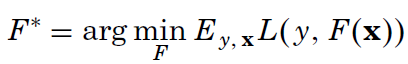
We search for the F* function that minimizes the average loss, given the past input (x is a vector), and y (a scalar output). The article explores three different loss functions; among them the usual square-error and the Huber loss function – something new to me and here is its definition:

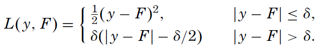
The author has chosen this function because he is looking for an highly robust learning procedure: if the difference between the predicted output and the real one is smaller than delta, it is used, otherwise just the error direction is taken into account. In this way the procedure will discard outliers. Of course, using the Huber loss function, you need to decide the delta value.

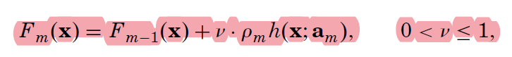
But how do you search for F*? We will not look for whatever function, but we will restrict the search to a function family, regression trees. The single functions will be identified by a parameter set a={a_1,a_2…}. With XGBoost we were adding one new regression tree at each learning step, this comes from the way the gradient boosting searches for F*: additive expansion

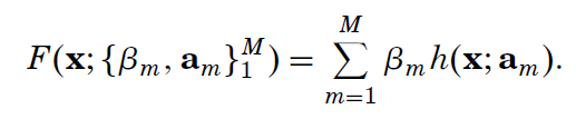
At each leaning step m, a new simple function beta_m*h(x1,…,a_1,…,a_m) is added to the previous approximation: in this way a more and more complex function is built. The prediction will not diverge, as the added function produces positives or negatives values. This method is very powerful! This is the author’s explanation:

Such expansions (2) are at the heart of many function approximation methods such as neural networks [Rumelhart, Hinton, and Williams (1986)], radial basis functions [Powell (1987)], MARS [Friedman (1991)], wavelets [Donoho(1993)] and support vector machines [Vapnik (1995)]. Of special interest here is the case where each of the functions h(x,a_m) is a small regression tree,
such as those produced by CART TM [Breiman, Friedman, Olshen and Stone (1983)]. For a regression tree the parameters a_m are the splitting variables, split locations and the terminal node means of the individual trees.

How do you choose the next beta_m*h(x1,…,a_1,…,a_m)? You chose the best function that minimize the Loss function: with appropriate function this corresponds to calculate a derivative, and find the parameters that makes this value zero, to find its minimum. The article becomes dense of math and statistics, as you have a finite set of inputs, and regression trees are not really function where you can calculate a derivative! I really miss a lot of theory to understand the paper.

The paper describes a generic algorithm that must be adapted to different loss functions to be used.

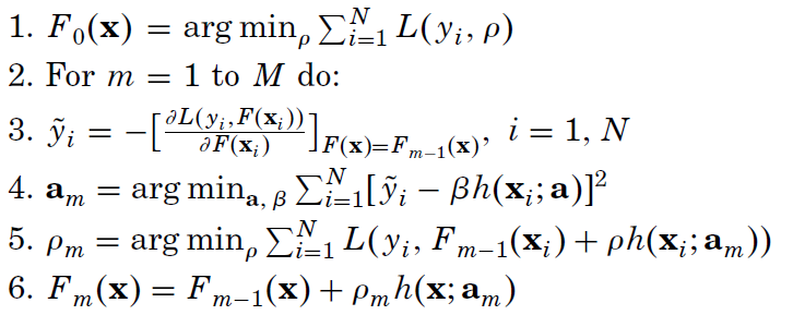
You start from an F_0 initial approximation, at each new step you calculate y~ given the past knowledge. You search then the best h_m that tries to match the optimal gradient descend and you choose the optimal weight rho to add h_m to the additive expansion.

The article continues deriving the correct algorithms to use with different loss functions and the introduces the “regularization”. Practical experience suggest to introduce a learning rate v constant, that is used to scale down the influence of new learned trees.

To apply the algorithm then you will have to choose the good M and v values. The article continues presenting some simulations and suggestion on which loss function to chose and how to choose these parameters. Another important parameter identified is J: the terminal nodes allowed to be in the regression trees. A too low J does not allow to learn complex relations, a too high value opens the door to over-fitting.