Giovanni Bricconi

I continued watching

Machine Learning Algorithms in 7 Days By Shovon Sengupta

Video link

And this time the subject was Logistic Regression; having caught cold did not help studying this week, sob. Here are my notes

This is the sigmoid function 1/(1+e^-x), as you can see it goes from 0 to 1, and at x=0 it’s value is 1/2. This function will be used to classify the inputs to two categories 0 or 1, no or yes. Once trained the model, it will be evaluated with the inputs, and the sigmoid will be computed. If the result is closer to 0 then the category 0 will be chosen, otherwise the category will be 1. So logistic regression can by tried whenever you have a binary classification problem, such as will this customer subscribe a new contract?

With a trick it is be possible to extend it to multiple categories: suppose you want to classify the inputs into 3 categories A,B, and C. You can formulate 3 binary questions: is it A or something else? is it B or something else… You can then train 3 logistic model, and each of them will predict an y value, you will chose the category that has the highest y value as the correct category (softmax).

The actual formulation does not use directly the sigmoid, but a logarithm of probabilities. Let’s be p the category 1 probability, the logit function is defined as ln[p / (1-p) ]. The model that will be trained will obey to this equation:

So you can have as many explanatory variables X as you want. The training process will identify the theta coefficients that minimize the classification error.

As for the linear regression, the training continues presenting a plethora of statistic indexes to judge the trained model: concordance, deviance, Somer’s D, C statistic, divergence, likelihood ratio, Wald chi-square… Luckily the sample code can be used to understand practically what to do in a Jupyter Notebook: https://github.com/PacktPublishing/Machine-Learning-Algorithms-in-7-Days/blob/master/Section%201/Code/MLA_7D_LGR_V2.ipynb

The samples contains examples on:

• Identify categorical variables, and how to generate dummy variables to be used in the training
• How to plot frequence histograms, to explore the data
• How to produce boxplots, to understand data distribution
• Using the describe function to get avg, stddev and quantile distributions
• Using Recursive Feature Elimination, to select only the most relevant explanatory variables
• Using MinMax scalers to prepare the data and how to train the logistic regression model
• Check for multi-collinearity and further reduce the used explanatory variables
• Plot the model’s ROC (receiver operating characteristic)
• Plot a Shap diagram to understand which are the most relevant libraries and how they influence the classifier.

This week I have been suggested to watch this video:

Machine Learning Algorithms in 7 Days

Video link

By Shovon Sengupta

It’s 5 hours and a half video on machine learning algorithms, authored by a principal data scientist at Fidelity Investments. Of course I did not have 5 hours spare time this week to follow it all, I just started watching the first “chapter” on linear regression. Shovon Sengupta made the subject passionating adding a lot of references to statistic tests. Actually the chapter goes so fast that you need to take some extra time searching explanations and definitions to understand better. Luckily there is support material, and you have access to a git report with the Jupyter notebooks used, so you can read them an test them later.

So what is the recipe to cook a linear regression?

• Clean the input data: check for missing data and decide what to do with outliers as the linear regression will be influenced by them. I hope that for outliers there will be another section in the video because in this part it went too quick – but in the sample there is at least one suggestion
• Check for multi-collinearity: this is interesting and well explained. It may happen that some of the input variables (explanatory variables) have a linear correlation between them, so they are not really independent. To make an absurd example you can have two input columns, one in the temperature in Fahrenheit degrees and the other in Celsius degrees. You must not use both of them or the linear regression algorithm may not work well.
• Select the features: you should analyze the explanatory variables to decide which ones to use, those that have more influence on the output variable. The training explains the Ridge and LASSO methods.
• Build the model on some training data
• Validate the model performance on test data.

So, even if it is just a linear regression, to do it well you need to do many not obvious things. Here I list for myself many definitions that are needed to understand the samples provided in the training

R2 explains the proportion of variance explained by the model

So the sum of squared prediction errors divided by the error you have pretending that the model is just the constant average value

You can have a better adjusted R2 index, taking into account the number of samples you have n and the number of input variable you use p:

You use R2 to calculate the variance inflation factor that is just 1/(1-R2) and it is an indicator useful to check if there is multicollienarity. The lower the better

The F statistic to check if there is a good relationship between the predicted output and the chosen explanatory variables. The higher the value the better is the relation.

The Durbin Watson test is instead used to test the presence of autocorrelation:

It will always have a value ranging between 0 and 4. A value of 2.0 indicates there is no autocorrelation detected in the sample. Values from 0 to less than 2 point to positive autocorrelation and values from 2 to 4 means negative autocorrelation. 

DW test statistic values in the range of 1.5 to 2.5 are relatively normal. Values outside this range could, however, be a cause for concern

From <https://www.investopedia.com/terms/d/durbin-watson-statistic.asp>

Another concept to check is the prediction error homoscedasticity: is the error just coming from a normal distribution or does it have an evolution? With the Breusch Pagan test you can check if the error

The last interesting concept is the regularization: the coefficients identified by the regression algorithm can tend to explode, or include variable that cause sample data overfitting. It is important to boost simpler models and this can be done introducing some penalty terms in the loss function

LassO  Least Absolute Shrinkage and Selection Operator,

Ridge

The lasso method has the advantage of removing low importance variables from the model, while the Ridge makes them very small but not zero. See <https://www.datacamp.com/tutorial/tutorial-lasso-ridge-regression> for a nice description.

But concretely how to use all these concepts? Luckily the training points to this git repository, where you have a nice python script that step by steps applies many of these checks on some sample data, and produces many graphs that helps understanding the concepts. https://github.com/PacktPublishing/Machine-Learning-Algorithms-in-7-Days/blob/master/Section%201/Code/MLA_7D_LR_V1.ipynb

Nothing easier than a linear regression? Not at all, if you don’t want just scratch the surface!

Last week I read about the XGBoost library and I wanted to understand more about the theory behind it. I started then reading this referenced article, and I have found a lot of explanations:

Jerome H. Friedman. “Greedy function approximation: A gradient boosting machine..” Ann. Statist. 29 (5) 1189 – 1232, October 2001. https://doi.org/10.1214/aos/1013203451

The document is very long, more than 40 pages, dense of math and statics; something too long to digest in my short weekly spare time. This is what I have learned so far. The goal of this method is to approximate an unknown function given the inputs and outputs collected in the past. This is very general, and requires a Loss function to be defined.

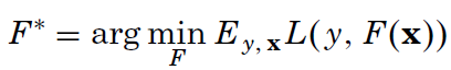
We search for the F* function that minimizes the average loss, given the past input (x is a vector), and y (a scalar output). The article explores three different loss functions; among them the usual square-error and the Huber loss function – something new to me and here is its definition:

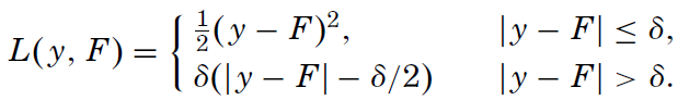
The author has chosen this function because he is looking for an highly robust learning procedure: if the difference between the predicted output and the real one is smaller than delta, it is used, otherwise just the error direction is taken into account. In this way the procedure will discard outliers. Of course, using the Huber loss function, you need to decide the delta value.

But how do you search for F*? We will not look for whatever function, but we will restrict the search to a function family, regression trees. The single functions will be identified by a parameter set a={a_1,a_2…}. With XGBoost we were adding one new regression tree at each learning step, this comes from the way the gradient boosting searches for F*: additive expansion

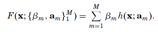
At each leaning step m, a new simple function beta_m*h(x1,…,a_1,…,a_m) is added to the previous approximation: in this way a more and more complex function is built. The prediction will not diverge, as the added function produces positives or negatives values. This method is very powerful! This is the author’s explanation:

Such expansions (2) are at the heart of many function approximation methods such as neural networks [Rumelhart, Hinton, and Williams (1986)], radial basis functions [Powell (1987)], MARS [Friedman (1991)], wavelets [Donoho(1993)] and support vector machines [Vapnik (1995)]. Of special interest here is the case where each of the functions h(x,a_m) is a small regression tree,
such as those produced by CART TM [Breiman, Friedman, Olshen and Stone (1983)]. For a regression tree the parameters a_m are the splitting variables, split locations and the terminal node means of the individual trees.

How do you choose the next beta_m*h(x1,…,a_1,…,a_m)? You chose the best function that minimize the Loss function: with appropriate function this corresponds to calculate a derivative, and find the parameters that makes this value zero, to find its minimum. The article becomes dense of math and statistics, as you have a finite set of inputs, and regression trees are not really function where you can calculate a derivative! I really miss a lot of theory to understand the paper.

The paper describes a generic algorithm that must be adapted to different loss functions to be used.

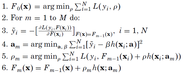
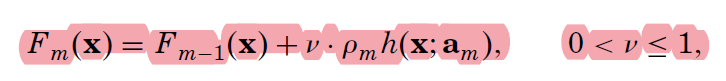
You start from an F_0 initial approximation, at each new step you calculate y~ given the past knowledge. You search then the best h_m that tries to match the optimal gradient descend and you choose the optimal weight rho to add h_m to the additive expansion.

The article continues deriving the correct algorithms to use with different loss functions and the introduces the “regularization”. Practical experience suggest to introduce a learning rate v constant, that is used to scale down the influence of new learned trees.

To apply the algorithm then you will have to choose the good M and v values. The article continues presenting some simulations and suggestion on which loss function to chose and how to choose these parameters. Another important parameter identified is J: the terminal nodes allowed to be in the regression trees. A too low J does not allow to learn complex relations, a too high value opens the door to over-fitting.