Giovanni Bricconi

After reading the short term weather forcast paper, I was curious about the LTSM and I dedided to learn about it. On wikipedia I have found a reference to this article:

LSTM: a search space odyssey. Klaus Greff, Rupesh K. Srivastava, Jan Koutnìk, Bas R. Steunebrink, Jurgen Schmidhuber. DOI: 10.1109/TNNLS.2016.2582924

It was nice to see that all the authors are from an university really close to my home town! The cv of Jurgen Schmidhuber is really impressive too.

Probably was not the best pick as article because it is not really about LSTM inception but it report on an huge experimentation of different variants, reporting and comparing theirs performances. By converse it has been interesting to see how they managed to fairly compare all these variants, and how they did the hyperparameters tuning.

But what are the LSTM neural networks for? Looking at the 3 use cases used to compare variants performance I see:

• recognising 61 different sound humans can pronounce. The used the TIMIT speach corpus

• recognising handwritten text. The IAM Online Handwriting Database contains hadwritten vector images and the ascii text corresponding to the picture. It is not just a picture as it contains also information on when the pen has been lifted.

• J. S. Bach Chorales, the machine learning model has to learn how harmonies are created. (https://axon.cs.byu.edu/Dan/673/papers/allan.pdf)

So all tasks where time evolution is very important.

The LSTM block itself it is really complicated! First of all there is not just input and output , there are four different input types: block input, plain input, forget gate input, and output gate input. These are taking as input not only the current input, but also the output at t-1. Internally a cell value c is computed and propagated with time delay to the forget gate and to the input gate, and without delay to the output gate; these connections are called peepholes. Finally there is an output block. Sorry, complex and difficult to describe.

The idea is that a memory cell maintains a state over time, and nonlinear gates regulates how information flow into and out of the cell. I reproduce here a similar picture to the one in the article to give an idea, but as the article is available on arxiv it is much better to check the original one directly at page 2.

In formulas:

z_t = nonlin(w_z x_t + r_z y_t-1 +b_z)

i_t = nonlin(w_i x_t + r_i y_t-1 + dot_product(p_i, c_t-1) +b_i)

f_t = nonlin(w_f x_t r_f y_t-1 + dot_product(p_f,c_t-1) + b_f)

c_t = dot_product(z_t, i_t) + dot_product(c_t-1, f_t)

o_t = nonlin( w_o x_t +r_o y_t-1 + dot_product(p_o, c_t) +b_o)

y_t = dot_product(nonlin(c_t) , o_t)

Where w and r are matrices of coefficents; b and p are real coefficients. So complex!

Forget gate is there to let the network learn when to reset itself; my understanding, concerning the handwritten example, the network can learn when a character is completed and a new one is starting, for instance when the text is written in italics. The peephole connextions were introduced to improve learning precise timings.

With a so complex schema it is clear that you can make many small changes to it, and question if that is an improvement or not. That is precisely the scope of the article: they compared the original model with 7 variants.

Since each variant had different schemas and different hyper-parameters, they had firt of all to identify the good seetting for each model and for each set of training data: an huge work but needed to ensure that you compare the best possible results that you can achieve with each model.

The variants compared are: no input gate (always =1), forget gate always 1, output gate always 1, no input activation formula (z(x) = x), no output activation formula (h(c_t) = c_t), coupling input and forget gate together f_t = 1 – i_t, removing peepholes, and full gate recurrence (many more coefficients to feed back in input values of i, f and o at t-1)

Often these changes are not so important, after the training the different networks reach more or less the same performances. This is not true if you remove the output activation function or the forget gate. So from the results those 2 components are very important. Coupling input and forget gates together does not hurt perfomances but reduces the parameters to learn, so seems a good idea to try it. The same for removing the peepholes. Notice also that the very complex full gate recurrence does not bring advantages.

Another interesting part of the article is about how they have tuned the hyper-parameters such as learning rate, momentum, adding gaussian input noise… They refer to the fANOVA framework, and it has let them taking some conlusion on how to tune these parameters.

The learning rate is the most important parameter, start with an high value and decrease it until performance stops increasing. Smaller values will not do better. Adding gaussian noise to the inputs was not useful and they have found that it is not requirend to invest much time in tuning the momentum, as it does not improve significatively the performance.

They also worked on understanding the influence of one hyperparameter on the other, and luckily they seems quite intependent so they can be tuned individually.

Reading some papers I frequently see these kinds of graphs. Since it’s long time I completed my studies, I have forgotten how to use them, and I need a refresh. Here you see one ROC curve taken from Machine Learning-based Short-term Rainfall Prediction from Sky Data. https://doi.org/10.1145/3502731

As usual, a quick look at wikipedia always helps: https://en.wikipedia.org/wiki/Receiver_operating_characteristic. There is a long list of indicator and a long discussion about other ways of selecting a model, a bit too compliaced to digest during a Saturday morning, but here are the key points.

Main assumption: you machine learning model answers a binary question, is there a dog in the picture, or will it rain in 30 minutes. In this context you will have a test set where you have input values and the correct classification label: int this picture there is a dog, in this one no (don’t care if there is a parrot).

I assume that, if your model need to classify pictures betwee dog, cats and parrots, you can end up having one ROC diagram for each class: this picture contains a dog, vs this picture contains a cat or a parrot.

I am pretty sure that, if you have many more classes, you end up with too many curves and this method is not useful anymore.

But to come back to the binary question, you have 4 possible situation for each sample

• the answer is yes and the ML model has found yes: True Positive (TP)
• the answer is no and the ML model has found yes: False Positive (FP)
• the answer is yes and the ML model has found no: False Negative (FN)
• the answer is no and the ML model has found no: True Negative (TN)

This makes things simple to understand, but for me it hides a par of the reasoning: usually ML models depends on parameters, for instance a threshold ML(x,y,z…) so the answer the model can give is a function of these parameters. So TP, FP… are actually TP(x,y,z..), FP(x,y,z..)…

So if you have only one parameter, say t for threshold, you have TP(t), FP(t), etc. As usual you can decide to plot these curves and try to guess the better threshold.

The ROC method tells you to plot together on a cartesian plan these 2 functions

FPR(t) = FP(t)/(FP(t)+TN(t)) fall-out or false positive rate

TPR(t) = TP(t)/(TP(t)+FN(t)) sensitivity, recall, hit-rate or true positive rate

So there are too many names for the same functions, this complicates the things when you read an article.

My conclusion is, if you have many parameters, that you just have to plot on the diagram a family of functions, and then chose the better parameters value to use it in your classification problem. But how do you choose them?

Check this picture on wikipedia: https://en.wikipedia.org/wiki/Receiver_operating_characteristic#/media/File:Roc_curve.svg

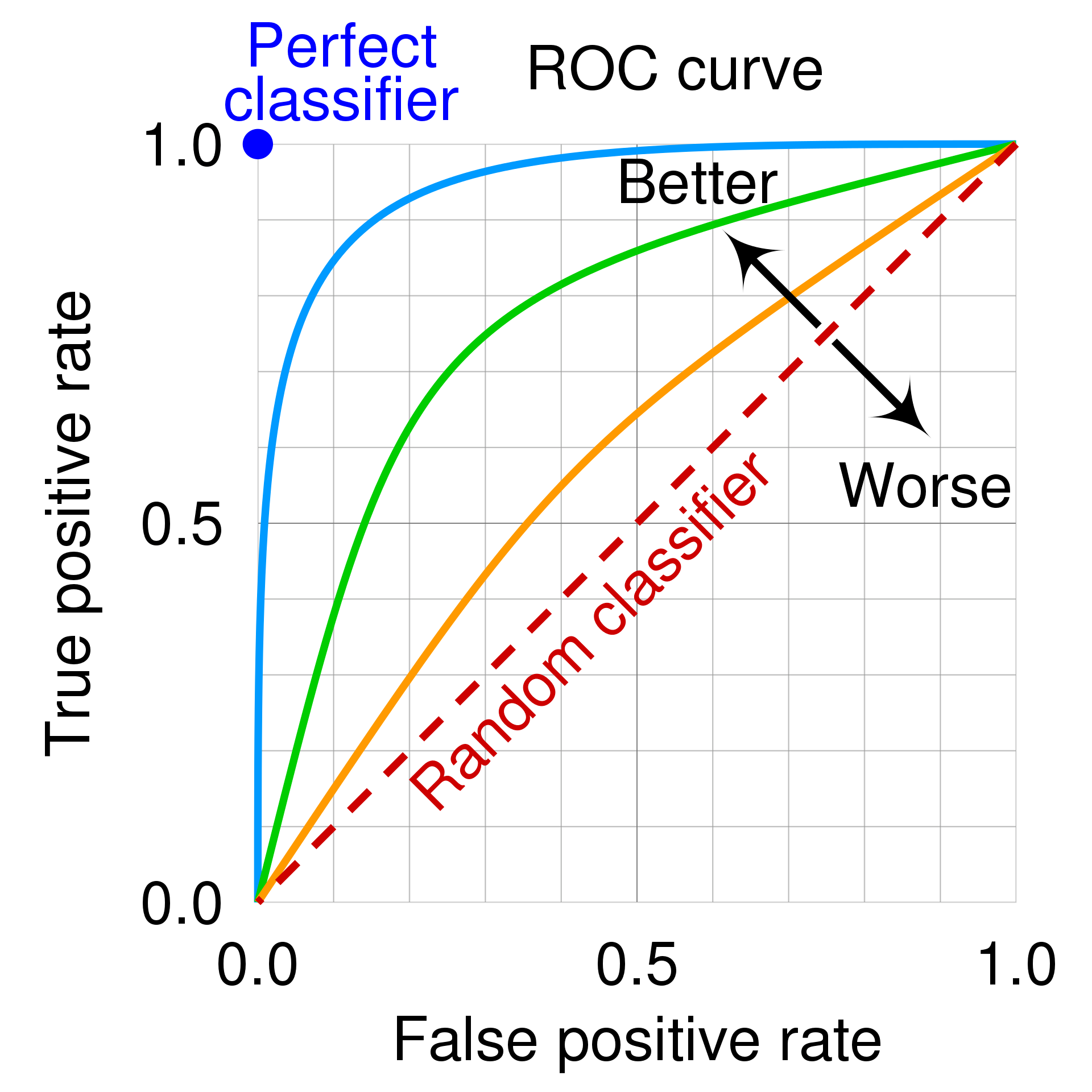
So the upper left corner is the perfect classfier, that is one that has true positive rate of 1: all yes prediction match perfectly the test data, and it has no false positive at all.

My guess is then that you just have to pick the point on your ROC curve that is more close to it and use those parameters.

In the pages I have seen it is always said that the diagonal is the response of a binary random variable: if your ROC curve is close to it, your model is as powerful as flipping one coin and say yes when you see the head, just useless. Also if your model is very bad, just replace yes with now, and you will have a better model (a test that always find that you don’t have covid, and never makes false predictions, would be indeed useful if you want to know if you have the covid).

So what was bothering me of many ROC curves plotted, like the one at the beginning of the page, is that there are no parameter values on the line, and this made me not understand how to actually use them.

This week I have found a nice article:

Fu Jie Tey, Tin-Yu Wu, and Jiann-Liang Chen. 2022. Machine Learning-based Short-term Rainfall Prediction from Sky Data. ACM Trans. Knowl. Discov. Data 16, 6, Article 102 (September 2022), 18 pages. https://doi.org/10.1145/3502731

I enjoyed reading it for various reasons. First of all, it gently introduces some terms and provides many pictures that let you familiarize with the needed concepts. We can guess the meaning of high accuracy, high precision, and recall rate, but it is much better to see the formulas that define them. This is concentrated in a couple of pages, it is a good reference. For instance, accuracy is defined as (# of true positive+true negative predictions)/(all predictions), and precision is just (# of true positive prediction)/(# of true or false positive predictions). Having these 2 pages greatly simplifies interpreting the results presented.

Then it describes how sky data has been acquired. They have deployed some Raspberry-pi modules, taking sky pictures, and also some Arduino-based weather sensors collecting temperature, UV rays, humidity, etc. They describe some difficulties encountered, and some workarounds used, for instance why they have chosen a particular angle when taking sky pictures.

For short-term prediction they mean answering the question: will it rain within 30 minutes? The purpose of the study was to see if a machine learning model, based on sky pictures and some other measures can be accurate enough. Usually, weather forecasts are made using complex mathematical models, on big computers, and their approach requires much less resources.

Their machine learning model is composed of a ResNet-152 convolutional neural network followed by a Long short-term memory recurrent neural network. It has been trained with about 60’000 images and has a recall of 87% on predicting rain absence and 81% on predicting rain.

This week I have decided to read an article about Neural Network interpretation: deep neural networks are made with many layer or many to many connected units, each having many parameters. Once trained they work well but the parameters are too many to understand what they mean, and we have to trust them as black boxes.

As humans we would like instead to have decision trees that we can review, to understand how the decision has been taken. The article I have read was about using neural networks to tune decision rules. You start the training with some expert-defined rules and after the training you get the same rules with better tuned parameters. So the expert can review them and see if they make sense.

The full reference to the article is: Xiaoyu Chen, Yingyan Zeng, Sungku Kang, and Ran Jin. 2022. INN: An Interpretable Neural Network for AI Incubation in Manufacturing. ACM Trans. Intell. Syst. Technol. 13, 5, Article 85 (June 2022), 23 pages. https://doi.org/10.1145/3519313

The idea is that human experts study a problem and are already able to provide some rules to classify the outcome of an experiment. The threshoulds that they set-up are probably sub optimal and they can be improved by some data driven algorithms. The paper refers to the case of crystal growth manufacturing: the expert have already identified some important parameters, such has heater power or pull speed, and have provided an initial model. The model is expressed in term of rules like if x>5 and y<3 or i>6 and j>9 then the crystal is defective (the paper does not provide real rule examples).

What is proposed it to apply a process that translate the rules into a neural network. The particularity is that the layers are not fully connected, but in some layers connections are made just where the input variables are related by model rules. In their case the proposal is to use 4 layers, some rules are provided to help applying the method to different cases.

Once the network is configured, a classical training algorithms can be used
to tune it, and obtain better thresholds in the rules. Notice that they propose
to use a special activation function, called Ca-Sigmoid, to allow incorporating
thresholds in the neural network; this just for the input layer.

Of course the limitation is that the learning process will not learn new rules, it will only optimize the existing ones.